Activation Functions - From Neuron to GPT

So far we have focused on the linear regression part of the network model and set aside the activation function of the M-P neuron model.

In theory, if we only use linear regression, a network model with any number of layers is still a linear transformation and is not fundamentally different from a single-layer network model. This is exactly what we observed in the previous chapter.

💡 Tip: According to the universal approximation theorem, it has been mathematically proven that, under certain conditions, a network model with at least one hidden layer and a nonlinear activation function can approximate any continuous function to arbitrary precision.

To make a neural network truly powerful, we must introduce nonlinearity. This is what an activation function does. Using activation functions between linear layers frees the network model from being limited to linear models, so that it can learn more complex relationships between inputs and outputs.

The activation function is part of the artificial neuron. In deep learning practice, however, it is usually designed as a separate layer that works together with the linear layers.

from abc import ABC, abstractmethod

import numpy as np

np.random.seed(42)

Tensor¶

class Tensor:

    def __init__(self, data):
        self.data = np.array(data)
        self.grad = np.zeros_like(self.data)
        self.gradient_fn = None
        self.parents = set()

    def backward(self):
        if self.gradient_fn is not None:
            self.gradient_fn()

        for p in self.parents:
            p.backward()

    def __str__(self):
        return f'Tensor({self.data})'

Dataset¶

class Dataset:

    def __init__(self, batch_size=1):
        self.batch_size = batch_size
        self.load()
        self.train()

    def load(self):
        self.train_data = ([[22.5, 72.0],
                            [31.4, 45.0],
                            [19.8, 85.0],
                            [27.6, 63.0]],
                           [[95],
                            [210],
                            [70],
                            [155]])
        self.test_data = ([[28.1, 58.0]],
                          [[165]])

    def train(self):
        self.data = self.train_data

    def eval(self):
        self.data = self.test_data

    def all(self):
        x, y = self.data
        return Tensor(x), Tensor(y)

    def __len__(self):
        x, *_ = self.data
        return len(x) // self.batch_size

    def __getitem__(self, index):
        s = slice(index * self.batch_size, (index + 1) * self.batch_size)
        x, y = self.data
        return Tensor(x[s]), Tensor(y[s])

Model¶

Abstract layer¶

class Layer(ABC):

    def __call__(self, x: Tensor):
        return self.forward(x)

    @abstractmethod
    def forward(self, x: Tensor):
        pass

    @property
    def parameters(self):
        return []

Linear layer¶

class Linear(Layer):

    def __init__(self, in_size, out_size):
        self.weight = Tensor(np.random.randn(out_size, in_size) * np.sqrt(2 / in_size))
        self.bias = Tensor(np.zeros(out_size))

    def forward(self, x: Tensor):
        p = Tensor(x.data @ self.weight.data.T + self.bias.data)

        def gradient_fn():
            self.weight.grad += p.grad.T @ x.data
            self.bias.grad += np.sum(p.grad, axis=0)
            x.grad += p.grad @ self.weight.data

        p.gradient_fn = gradient_fn
        p.parents = [x]
        return p

    @property
    def parameters(self):
        return [self.weight, self.bias]

Sequential layer¶

class Sequential(Layer):

    def __init__(self, layers):
        self.layers = layers

    def forward(self, x: Tensor):
        for l in self.layers:
            x = l(x)
        return x

    @property
    def parameters(self):
        return [p for l in self.layers for p in l.parameters]

Activation functions¶

Rectified linear unit (ReLU)¶

The rectified linear unit (ReLU) is the most commonly used activation function for intermediate hidden layers. Its logic is very simple: negative numbers become zero.

The advantages of the ReLU activation function are obvious:

it is computationally efficient and only needs a threshold operation;
it filters out all negative numbers. This can be understood as filtering out all the unimportant information, or noise;
all positive numbers stay unchanged, and the derivative is always 1 in the positive range. So it does not weaken useful information and avoids vanishing gradients. This is essential for training deep networks.

Forward propagation: negative numbers are set to zero.

y = \text{ReLU}(x) = \max(0, x)

(1)

Gradient computation: positive numbers keep their gradient. The derivative of the ReLU activation function is:

\frac{dy}{dx} = \begin{cases} 1 & \text{if } x > 0 \\ 0 & \text{if } x \leq 0 \end{cases}

(2)

Parent list (parents): the input.

Parameter list (parameters): none, because there are no parameters to train.

class ReLU(Layer):

    def forward(self, x: Tensor):
        # Create the activation tensor
        a = Tensor(np.maximum(0, x.data))

        # Gradient (closure) function of the activation tensor
        def gradient_fn():
            x.grad += a.grad * (a.data > 0)

        a.gradient_fn = gradient_fn
        # Parent list of the activation tensor
        a.parents = [x]
        return a

Let’s look at the effect of the ReLU activation function:

import matplotlib.pyplot as plt

relu = ReLU()

plt.figure(figsize=(5, 3))
x_range = np.arange(-10, 10, 0.1)
plt.plot(x_range, [relu(Tensor(x)).data for x in x_range], linewidth=2)
plt.xlabel('x', fontsize=12)
plt.ylabel('y', fontsize=12)
plt.title('ReLU', fontsize=14, fontweight='bold')
plt.grid(True, alpha=0.3)
plt.tight_layout()
plt.show()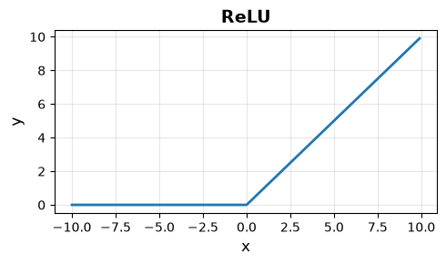

Hyperbolic tangent (Tanh)¶

The hyperbolic tangent (Tanh) maps any value into the range $(-1, 1)$ while preserving the relative relationships between values. It can be used to remove extreme values caused by “overexposure” and center the data around zero. Like the ReLU activation function, it is commonly used in intermediate hidden layers.

Forward propagation: the hyperbolic tangent maps the input into the range $(-1, 1)$ . The output is zero-centered (its mean is 0). We simply call the tanh function provided by NumPy to compute it.

y = \tanh(x) = \frac{e^x - e^{-x}}{e^x + e^{-x}}

(3)

Gradient computation: the derivative of the Tanh activation function can be expressed with the function itself. This means we do not need to compute the complicated exponential functions again. The derivative of the Tanh activation function is:

\frac{dy}{dx} = 1 - \tanh^2(x) = 1 - y^2

(4)

When the input is very large or very small, the derivative approaches 0. This is what we usually call gradient saturation. In deep networks, it makes the signal passed back weaker and weaker, and eventually leads to vanishing gradients.

Parent list (parents): the input.

Parameter list (parameters): none.

class Tanh(Layer):

    def forward(self, x: Tensor):
        # Create the activation tensor
        a = Tensor(np.tanh(x.data))

        # Gradient (closure) function of the activation tensor
        def gradient_fn():
            x.grad += a.grad * (1 - a.data ** 2)

        a.gradient_fn = gradient_fn
        # Parent list of the activation tensor
        a.parents = [x]
        return a

Let’s look at the effect of the Tanh activation function:

tanh = Tanh()

plt.figure(figsize=(5, 3))
x_range = np.arange(-10, 10, 0.1)
plt.plot(x_range, [tanh(Tensor(x)).data for x in x_range], linewidth=2)
plt.xlabel('x', fontsize=12)
plt.ylabel('y', fontsize=12)
plt.title('Tanh', fontsize=14, fontweight='bold')
plt.grid(True, alpha=0.3)
plt.tight_layout()
plt.show()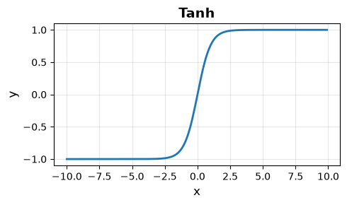

Sigmoid¶

The sigmoid function (also called the logistic curve) smoothly squashes any value into the range $(0, 1)$ . The output can therefore be interpreted as the probability of an event, and it is commonly used in the output layer of binary classification problems to regularize the prediction.

Forward propagation: the probability of logistic regression, mapping any real number into the interval $(0, 1)$ . Commonly used in the output layer of binary classification problems.

y = \sigma(x) = \frac{1}{1 + e^{-x}}

(5)

Gradient computation: the derivative of the Sigmoid activation function can also be expressed with the function itself. The derivative of the Sigmoid activation function is:

\frac{dy}{dx} = \sigma(x) \cdot (1 - \sigma(x)) = y(1 - y)

(6)

The Sigmoid activation function also suffers from gradient saturation. In deep networks, the gradient may vanish. In addition, the Sigmoid activation function suffers from gradient decay.

Parent list (parents): the input.

Parameter list (parameters): none.

class Sigmoid(Layer):

    def __init__(self, clip_range=(-100, 100)):
        super().__init__()
        self.clip_range = clip_range

    def forward(self, x: Tensor):
        # Clip the values to prevent overflow
        z = np.clip(x.data, self.clip_range[0], self.clip_range[1])
        # Create the activation tensor
        a = Tensor(1 / (1 + np.exp(-z)))

        # Gradient (closure) function of the activation tensor
        def gradient_fn():
            x.grad += a.grad * a.data * (1 - a.data)

        a.gradient_fn = gradient_fn
        # Parent list of the activation tensor
        a.parents = [x]
        return a

Let’s look at the effect of the Sigmoid activation function:

sigmoid = Sigmoid()

plt.figure(figsize=(5, 3))
x_range = np.arange(-10, 10, 0.1)
plt.plot(x_range, [sigmoid(Tensor(x)).data for x in x_range], linewidth=2)
plt.xlabel('x', fontsize=12)
plt.ylabel('y', fontsize=12)
plt.title('Sigmoid', fontsize=14, fontweight='bold')
plt.grid(True, alpha=0.3)
plt.tight_layout()
plt.show()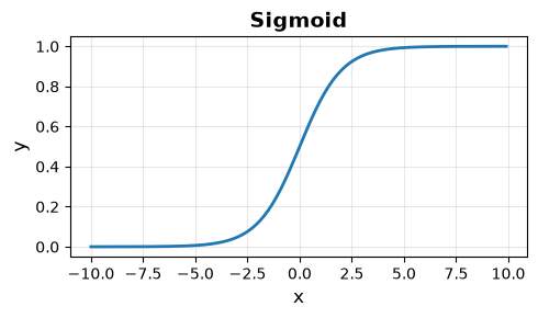

Softmax¶

The softmax function (normalized exponential function) works on a group of values: it converts them into relative proportions of one another and keeps the total at 1. It is therefore commonly used in the output layer of multi-class classification problems, where the option with the largest value is the prediction.

Forward propagation: maps any real vector to a probability distribution, so that every component lies in the interval $(0, 1)$ and all the components sum to 1. Commonly used in the output layer of multi-class classification problems.

y_i = \frac{e^{x_i}}{\sum_{j=1}^{n} e^{x_j}}

(7)

Gradient computation: the Softmax activation function is a vector function, and its gradient is a Jacobian matrix. The derivative of the Softmax activation function is:

\frac{\partial L}{\partial x_i} = y_i (g_i - \sum_{j=1}^{n} y_j g_j)

(8)

Where:

$y_i$ : the $i$ -th output of Softmax;
$g_i$ : the gradient of the loss with respect to the $i$ -th output, that is, the gradient passed back from the next layer;
$n$ : the number of components of the vector.

The meaning of this formula is intuitive: first compute the average gradient weighted by all the output probabilities, then output the difference between each component’s gradient and the average gradient.

Parent list (parents): the input.

Parameter list (parameters): none.

class Softmax(Layer):

    def __init__(self, axis=-1):
        super().__init__()
        self.axis = axis

    def forward(self, x: Tensor):
        # Create the activation tensor
        exp = np.exp(x.data - np.max(x.data, axis=self.axis, keepdims=True))
        a = Tensor(exp / np.sum(exp, axis=self.axis, keepdims=True))

        # Gradient (closure) function of the activation tensor
        def gradient_fn():
            grad = np.sum(a.data * a.grad, axis=self.axis, keepdims=True)
            x.grad += a.data * (a.grad - grad)

        a.gradient_fn = gradient_fn
        # Parent list of the activation tensor
        a.parents = [x]
        return a

Let’s look at the effect of the Softmax activation function:

softmax = Softmax()

x_range = np.arange(-10, 10, 0.1)
plt.figure(figsize=(5, 3))
plt.plot(x_range, [softmax(Tensor([x, 0.1, 0.9])).data for x in x_range], linewidth=2)
plt.xlabel('x', fontsize=12)
plt.ylabel('y', fontsize=12)
plt.title('Softmax', fontsize=14, fontweight='bold')
plt.grid(True, alpha=0.3)
plt.tight_layout()
plt.legend(['x', '0.1', '0.9'])
plt.show()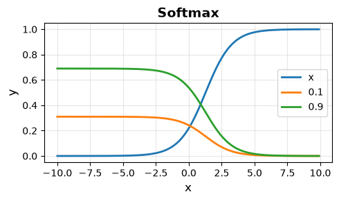

The Softmax activation function is a vector function, so we can see how its components relate to one another.

The figure compares the variable $x$ with two constants, 0.1 and 0.9, after they pass through the Softmax activation function. We can see that when $x$ is less than 0.9, the best choice is always 0.9; when $x$ is greater than 0.9, the best choice becomes $x$ ; and 0.1 is never the best choice.

Loss function (mean squared error)¶

class MSELoss:

    def __call__(self, p: Tensor, y: Tensor):
        return self.loss(p, y)

    def loss(self, p: Tensor, y: Tensor):
        mse = Tensor(np.mean(np.square(y.data - p.data)))

        def gradient_fn():
            p.grad += -2 * (y.data - p.data) / y.data.size

        mse.gradient_fn = gradient_fn
        mse.parents = [p]
        return mse

Optimizer (stochastic gradient descent)¶

class SGDOptimizer:

    def __init__(self, parameters, lr):
        self.parameters = parameters
        self.lr = lr

    def zero_grad(self):
        for p in self.parameters:
            p.grad = np.zeros_like(p.data)

    def step(self):
        for p in self.parameters:
            p.data -= p.grad * self.lr

Trainer¶

class Trainer:

    def __init__(self, model, loss_fn, optimizer):
        self.model = model
        self.loss_fn = loss_fn
        self.optimizer = optimizer

    def train(self, dataset, epochs):
        dataset.train()

        for epoch in range(epochs):
            for i in range(len(dataset)):
                feature, label = dataset[i]

                self.optimizer.zero_grad()
                prediction = self.model(feature)
                loss = self.loss_fn(prediction, label)
                loss.backward()
                self.optimizer.step()

    def test(self, dataset):
        dataset.eval()

        feature, label = dataset.all()
        prediction = self.model(feature)
        loss = self.loss_fn(prediction, label)
        return prediction, loss

Hyperparameters¶

Learning rate¶

LEARNING_RATE = 0.00001

Batch size¶

BATCH_SIZE = 2

Number of epochs¶

EPOCHS = 1000

Modeling¶

Now let’s apply the ReLU activation function after the hidden layer and see what effect it has.

💡 Tip: In regression models that predict numerical values, no activation function is usually needed after the output layer. Later we will see that in classification models, an activation function is also used after the output layer to help with the decision.

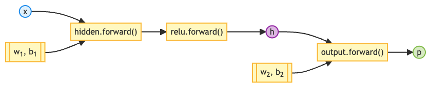
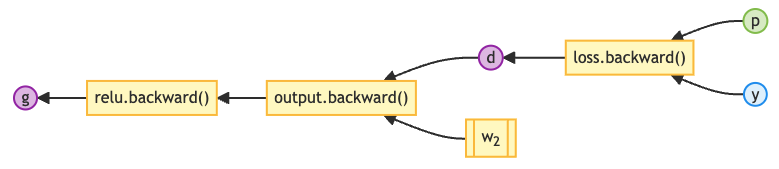
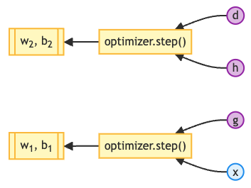
With the hidden layer activation function, the three core processes of the model change a little (the parameter update does not change):

Forward propagation:

Forward propagation with the ReLU layer: the feature x goes through hidden.forward() (parameters w₁, b₁) and relu.forward() to produce the intermediate value h, and then through output.forward() (parameters w₂, b₂) to produce the prediction p

Figure: Forward propagation (model inference)

Backpropagation:

Backpropagation with the ReLU layer: loss.backward() computes the error term d from the prediction p and the label y, and output.backward() (using w₂) and relu.backward() then produce the gradient g

Figure: Backpropagation (gradient computation)

Parameter update:

Parameter update in the two-layer network: optimizer.step() updates w₂ and b₂ from the error term d and the intermediate value h, and updates w₁ and b₁ from the gradient g and the feature x

Figure: Parameter update

dataset = Dataset(BATCH_SIZE)
model = Sequential([
    # Hidden layer
    Linear(2, 4),
    # Hidden layer activation function
    ReLU(),
    # Output layer
    Linear(4, 1)
])
loss_fn = MSELoss()
optimizer = SGDOptimizer(model.parameters, lr=LEARNING_RATE)
trainer = Trainer(model, loss_fn, optimizer)

Training¶

trainer.train(dataset, EPOCHS)

Evaluation¶

prediction, loss = trainer.test(dataset)
print(f'prediction:\t{prediction}\nloss:\t{loss}')

prediction:	Tensor([[164.60610313]])
loss:	Tensor(0.15515474192848927)

In the previous chapter, we observed that the two-layer network model worked, but did not perform better than the single-layer model and was even slightly worse.

After we add the hidden layer activation function, however, the loss drops to 0.16, close to 0.

This shows that after introducing a nonlinear activation function, the model has a stronger expressive power: it fits the training data well and gives reasonable predictions on the test sample.

Summary¶

The four activation functions compare as follows:

Activation function	Main use	Advantages	Disadvantages	Recommended position
ReLU	Default first choice Handles nonlinear features	Fast to compute No gradient saturation in the positive range Mitigates vanishing gradients	Zero gradient in the negative range Neurons may “die permanently”	Hidden layers
Tanh	Data with positive and negative values	Zero-centered output (mean 0) Makes the next layer converge faster	Gradient saturation Exponentials are expensive to compute	Hidden layers
Sigmoid	Probability prediction for binary classification	Smoothly squashes the output into $(0, 1)$ Output can be interpreted as a probability	Output mean is not 0 Severe gradient saturation Causes vanishing gradients	Binary classification output layer
Softmax	Probability prediction for multi-class classification	Handles the probabilities of several classes Ensures the probabilities sum to 1	Complex to compute Sensitive to extreme values	Multi-class classification output layer

Exercises¶

Try Tanh as the activation function, or use Sigmoid or Softmax after the output layer, and see how the training results change.