In deep learning, no matter which gradient descent method is used, one complete pass over the whole training set is called an epoch.
If the training set has samples:
Stochastic gradient descent: iterations per epoch;
Batch gradient descent: only 1 iteration per epoch;
Mini-batch gradient descent (batch size ): iterations per epoch.
Usually, a network model needs to be trained for multiple epochs before its parameters converge sufficiently to a good state.
import numpy as npTensor
class Tensor:

    def __init__(self, data):
        self.data = np.array(data)
        self.grad = np.zeros_like(self.data)
        self.gradient_fn = None
        self.parents = set()

    def backward(self):
        if self.gradient_fn is not None:
            self.gradient_fn()

        for p in self.parents:
            p.backward()

    def __str__(self):
return f'Tensor({self.data})'Dataset
class Dataset:

    def __init__(self, batch_size=1):
        self.batch_size = batch_size
        self.load()
        self.train()

    def load(self):
        self.train_data = ([[22.5, 72.0],
                            [31.4, 45.0],
                            [19.8, 85.0],
                            [27.6, 63.0]],
                           [[95],
                            [210],
                            [70],
                            [155]])
        self.test_data = ([[28.1, 58.0]],
                          [[165]])

    def train(self):
        self.data = self.train_data

    def eval(self):
        self.data = self.test_data

    def all(self):
        x, y = self.data
        return Tensor(x), Tensor(y)

    def __len__(self):
        x, *_ = self.data
        return len(x) // self.batch_size

    def __getitem__(self, index):
        s = slice(index * self.batch_size, (index + 1) * self.batch_size)
        x, y = self.data
return Tensor(x[s]), Tensor(y[s])Model
class Linear:

    def __init__(self, in_size, out_size):
        self.weight = Tensor(np.ones((out_size, in_size)) / in_size)
        self.bias = Tensor(np.zeros(out_size))

    def __call__(self, x: Tensor):
        return self.forward(x)

    def forward(self, x: Tensor):
        p = Tensor(x.data @ self.weight.data.T + self.bias.data)

        def gradient_fn():
            self.weight.grad += p.grad.T @ x.data
            self.bias.grad += np.sum(p.grad, axis=0)

        p.gradient_fn = gradient_fn
        return p

    @property
    def parameters(self):
        return [self.weight, self.bias]
Loss function (mean squared error)
class MSELoss:

    def __call__(self, p: Tensor, y: Tensor):
        return self.loss(p, y)

    def loss(self, p: Tensor, y: Tensor):
        mse = Tensor(np.mean(np.square(y.data - p.data)))

        def gradient_fn():
            p.grad += -2 * (y.data - p.data) / y.data.size

        mse.gradient_fn = gradient_fn
        mse.parents = [p]
        return mse
Optimizer (stochastic gradient descent)
class SGDOptimizer:

    def __init__(self, parameters, lr):
        self.parameters = parameters
        self.lr = lr

    def zero_grad(self):
        for p in self.parameters:
            p.grad = np.zeros_like(p.data)

    def step(self):
        for p in self.parameters:
p.data -= p.grad * self.lrTrainer
With the introduction of iterations, batch processing, and epochs, the code for model training and evaluation gradually becomes more complex. We encapsulate it into a trainer so that it can be reused across projects.
The most basic trainer provides two functions:
train(training method): the training method takes two parameters, the dataset and the number of epochs. It uses the training set of the dataset and runs the specified number of epochs of iterative training.test(test method): the test method takes one parameter, the dataset. It uses the test set of the dataset to run one round of testing on the trained model.
💡 Tip: Look at the training method of the trainer. Its core is exactly the “five-step loop” we saw before (zero the gradients, forward propagation, compute the loss, backpropagation, update the parameters), just wrapped in an additional epoch loop.
class Trainer:

    def __init__(self, model, loss_fn, optimizer):
        self.model = model
        self.loss_fn = loss_fn
        self.optimizer = optimizer

    # Training method
    def train(self, dataset, epochs):
        # Use the training set
        dataset.train()

        # Epoch
        for epoch in range(epochs):
            # Iteration
            for i in range(len(dataset)):
                feature, label = dataset[i]

                self.optimizer.zero_grad()
                prediction = self.model(feature)
                loss = self.loss_fn(prediction, label)
                loss.backward()
                self.optimizer.step()

    # Test method
    def test(self, dataset):
        # Use the test set
        dataset.eval()

        feature, label = dataset.all()
        prediction = self.model(feature)
        loss = self.loss_fn(prediction, label)
return prediction, lossLEARNING_RATE = 0.00001Batch size
BATCH_SIZE = 2Number of epochs
This is our third hyperparameter. The number of epochs defines how many times the training data is iterated over during model training.
More epochs are not always better:
In the early stage of training, the model parameters usually converge quickly as the epochs increase, and the error drops sharply;
After that, convergence gradually levels off;
If there are too many epochs, the model may overfit, and its performance in real use may even get worse.
So we need to monitor how the network model performs on the test data and find the turning point where the performance improvement stops. This determines the best number of epochs:
too few epochs: underfitting;
too many epochs: possible overfitting.
An effective practical technique is called early stopping: after each epoch, compare with the previous epoch. If the decrease in the loss is already very small (for example, less than 1%), the model has basically converged, and we can stop training early to avoid overfitting.
Another related technique is called shuffling: in every epoch, shuffle the order in which the training data are iterated, in the hope of optimizing the training further and getting better generalization.
EPOCHS = 1000Modeling
We pass the instances of the model, the loss function, and the optimizer to the trainer as parameters.
dataset = Dataset(BATCH_SIZE)
model = Linear(2, 1)
loss_fn = MSELoss()
optimizer = SGDOptimizer(model.parameters, lr=LEARNING_RATE)
trainer = Trainer(model, loss_fn, optimizer)Training
With a trainer, model training only requires calling the trainer’s training method.
trainer.train(dataset, EPOCHS)Evaluation
Likewise, evaluation only requires calling the trainer’s test method.
prediction, loss = trainer.test(dataset)
print(f'prediction:\t{prediction}\nloss:\t{loss}')
prediction: Tensor([[163.52327795]])
loss: Tensor(2.1807080003283335)
After 1000 epochs, the loss has dropped to a single digit.
At this point, we can declare: the model has been trained successfully!
Loss curve
Finally, let’s monitor how the loss changes in every epoch, to get an intuitive feel for the training process and see where the turning point is.
We use the Matplotlib plotting library to show how the loss changes as the epochs increase.
import matplotlib.pyplot as plt

# Modeling
dataset = Dataset(BATCH_SIZE)
model = Linear(2, 1)
loss_fn = MSELoss()
optimizer = SGDOptimizer(model.parameters, lr=LEARNING_RATE)

# Training
losses = []
for epoch in range(EPOCHS):
    dataset.train()
    for i in range(len(dataset)):
        feature, label = dataset[i]

        optimizer.zero_grad()
        prediction = model(feature)
        loss = loss_fn(prediction, label)
        loss.backward()
        optimizer.step()

    dataset.eval()
    feature, label = dataset.all()
    prediction = model(feature)
    loss = loss_fn(prediction, label)
    losses.append(loss.data)

# Display
plt.figure(figsize=(5, 3))
plt.plot(losses, linewidth=2)
plt.xlabel('Epochs', fontsize=12)
plt.ylabel('MSE Loss', fontsize=12)
plt.title('Loss Curve', fontsize=14, fontweight='bold')
plt.grid(True, alpha=0.3)
plt.tight_layout()
plt.show()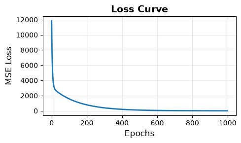
The figure above is the loss curve of model training. It shows intuitively how the loss drops quickly as the epochs increase and then gradually levels off.
Exercises
Try to implement early stopping during the iterations. Adjust the early stopping threshold (for example, 0.1%, 0.5%, 1%) and observe how it affects the number of epochs.
Try to implement shuffling during the iterations. Observe how it affects the loss.
Look at the loss curve above. Where do you think the turning point is?