Linear Regression - From Neuron to GPT

A tree thick enough to fill your arms grows from a tiny sprout; a nine-story tower rises from a heap of earth; a journey of a thousand miles begins at your feet.
Tao Te Ching, Chapter 64

Great achievements often begin with a simple idea.

Deep learning is no exception. It traces back to a remarkably simple mathematical model from 1943: the artificial neuron.

Artificial neurons¶

The human brain is not a single, monolithic processor. It is a complex network of about 86 billion neurons. A single neuron is very limited. It can only:

receive signals;
judge how strong the signals are;
decide whether to notify the next neuron.

Abstracted, this mechanism consists of input, weighting, filtering, and output.

Inspired by this, the neuroscientist Warren McCulloch and the logician Walter Pitts proposed the famous McCulloch-Pitts neuron (M-P neuron):

\text{output} = \begin{cases} 1 & \text{if } \sum\limits_{i=1}^{n} w_i x_i \geq \theta \\ 0 & \text{otherwise} \end{cases}

(1)

Where:

$x_i$ : the $i$ -th input value;
$w_i$ : the corresponding weight;
$\theta$ : the threshold;
$n$ : the number of inputs.

The model has two core ideas:

linear regression: compute a weighted sum of the inputs;
step function: filter the signal with a threshold $\theta$ to decide whether to pass it on.

💡 Tip: The original M-P model uses a step function. Modern deep learning instead uses a “continuously differentiable” activation function, which is what makes training with gradient descent possible.

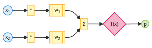
Structure of an artificial neuron: the inputs are multiplied by weights, summed, and passed through an activation function to produce the output

Figure: Structure of an artificial neuron

Where:

$x_1$ , $x_2$ : input values;
$w_1$ , $w_2$ : weights;
$p$ : the output value;
$f(x)$ : the activation function.

Neural networks¶

A single neuron is limited. But when we connect and stack thousands, even billions, of neurons into multiple layers, we get a powerful deep neural network (DNN). Multiple layers give a network far more flexibility. Each layer can combine the features from the previous layer into more abstract and more complex ones, and ultimately distill the underlying patterns in the data.

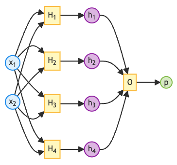
Structure of a two-layer neural network: two inputs, four first-layer neurons, and one second-layer neuron

Figure: Structure of a (two-layer) neural network

Where:

$x_1$ , $x_2$ : input values;
$H_1$ , $H_2$ , $H_3$ , $H_4$ : neurons in the first layer;
$h_1$ , $h_2$ , $h_3$ , $h_4$ : intermediate values;
$O$ : the neuron in the second layer;
$p$ : the output value.

Now let’s start from the simplest single-neuron model and build, step by step, an AI system that can understand language and generate content.

The simplest neural network model¶

A network with only one neuron is simple, yet it can already handle many practical tasks, such as:

trend prediction, for example forecasting house prices, stock prices, or sales;
impact analysis, for example health risk assessment or marketing attribution.

A single neuron does something very simple: it computes a weighted sum, which is also known as linear regression:

p = \sum_{i=1}^{n} w_i x_i + b

(2)

Where:

$x_i$ : the $i$ -th input, also called a feature;
$w_i$ : the corresponding weight;
$b$ : the bias;
$p$ : the result of the weighted sum, also called the prediction.

💡 Tip: A complete neuron model has two parts: linear regression and an activation function. In practice, the activation function is implemented separately and used together with the linear regression. We focus on the linear regression part first.

Let’s use an ice cream sales prediction problem as an example:

Ming runs an ice cream shop and has noticed that sales depend heavily on the weather. He wants to build a network model that predicts each day’s ice cream sales from the temperature and humidity.

import numpy as np

💡 Tip: NumPy is Python’s core library for scientific computing. It provides efficient multi-dimensional arrays (ndarray) and vectorized operations. We use NumPy for all the computations in this book.

Data¶

Features¶

Ming found today’s weather forecast, which gives us our first input data (also called features): a temperature of 28.1°C and a humidity of 58%.

We store today’s weather in a NumPy array: [temperature, humidity].

feature = np.array([28.1, 58.0])

Model¶

A model contains all the parameters (the weights and the bias) and the computation logic (the inference function) needed to make predictions.

Parameters: weights and bias¶

The number of weights matches the number of features. For example, the features $[x_1, x_2]$ contain two values (temperature and humidity), so we need exactly two weights: $[w_1, w_2]$ .

Weights represent how strongly each feature influences the prediction. For example, if $w_1$ is large and $w_2$ is small, people are buying ice cream mainly because of $x_1$ (hot weather) rather than $x_2$ (humid air).

The bias is a single number. It represents the baseline sales that do not depend on any feature, for example the steady purchases of die-hard ice cream lovers, who buy ice cream no matter the weather.

We also store the parameters in NumPy arrays:

Weights: a 2D array with shape (number of neurons, number of features). Each row holds all the weights of one neuron. The number of neurons equals the number of predictions, because each neuron produces one prediction.
Bias: a 1D array with shape (number of neurons,). Each value is the bias of one neuron.

Inference function¶

The inference function computes the weighted sum (linear regression). This flow of data from input to output is called forward propagation, so the inference function is also commonly called the forward function.

NumPy’s matrix operations let us implement linear regression efficiently:

p = \begin{bmatrix} x_1 & x_2 \end{bmatrix} \cdot \begin{bmatrix} w_1 \\ w_2 \end{bmatrix} + b

(3)

In code, x @ self.weight.T is equivalent to the matrix multiplication above. Here @ is the matrix multiplication operator, and self.weight.T is the transpose of the weight matrix. Transposing swaps its rows and columns, changing its shape from (1, 2) to (2, 1) so that the dimensions of the matrix multiplication match. The result is an array containing a single value, with shape (1,), which is exactly the prediction we want.

class Linear:

    def __init__(self, in_size, out_size):
        # Weights
        self.weight = np.ones((out_size, in_size)) / in_size
        # Bias
        self.bias = np.zeros(out_size)

    def __call__(self, x):
        return self.forward(x)

    # Inference function (forward propagation)
    def forward(self, x):
        return x @ self.weight.T + self.bias

💡 Tip: As initial values, we assume that temperature and humidity influence sales equally, so each weight is 0.5, and we set the bias to 0 because we do not yet know the baseline sales. Neither assumption is accurate. The goal of training is precisely to find better parameters automatically from data.

With just these few lines of code, we have built the simplest runnable neural network!

Modeling¶

Before running the model, we first need to create an instance of it: the input has 2 features and the output is 1 prediction.

model = Linear(2, 1)

Inference¶

Running a model instance to make a prediction is called model inference.

Now let’s have our model predict today’s ice cream sales for Ming.

prediction = model(feature)
print(f'prediction:\t{prediction}')

prediction:	[43.05]

The model predicts that Ming can sell about 43 ice creams today.

Is this prediction reliable? We will know the answer once the actual sales figures come in this evening.

Exercises¶

If we want to add more features (for example, wind speed), which parts of the model need to change, and how?