Automatic Differentiation - From Neuron to GPT

In the previous chapter, we used the chain rule of calculus to derive the gradients of the model parameters from the partial derivatives of the inference function and the loss function. In real applications, a network model may have dozens or hundreds of layers and millions or tens of millions of artificial neurons. For such a large, deep network, if we expand the chain rule separately for every parameter, the amount of computation explodes exponentially. So we need a mechanism that avoids repeated computation, differentiates the different basic operations automatically, and chains the derivatives together level by level according to each parameter’s position in the network.

The method used in deep learning is called the computational graph.

Computational graph¶

The computation of a neural network does not happen in one step. The input data passes through the neurons layer by layer, each step performing only a simple local operation, and finally converges in the loss function to produce the loss. This path along which data flows is forward propagation.

To be able to compute gradients, we need to record the whole topology of the data flow during forward propagation: which node’s output becomes the input of which node in the next layer. This recorded topology is called the computational graph.

Each node in the computational graph may be a feature, a model parameter, an intermediate result, or the final prediction or loss. The edges between nodes represent the direction of data flow and the dependencies. With the computational graph, we can trace backward along it and compute the gradient of each parameter level by level.

A computational graph built dynamically during forward propagation is called a dynamic computational graph. Its counterpart is the static computational graph, in which the whole structure of the graph is defined first and the data is fed in afterward. PyTorch uses dynamic computational graphs. Early versions of TensorFlow used static computational graphs (newer versions also support a dynamic mode). We will use dynamic computational graphs.

Now look back at our current network model with a single artificial neuron. Its complete computational graph looks like this:

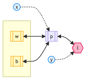
Computational graph of the single-neuron model: the feature, weight, and bias produce the prediction through the inference function, and the prediction together with the label produces the loss through the loss function

Figure: Computational graph

Where:

$x$ , $y$ : the feature and the label, leaf nodes that do not need training;
$w$ , $b$ : the weight and the bias, leaf nodes that need training;
$p$ : the prediction, an intermediate node;
$l$ : the loss, the root node.

import numpy as np

Tensor¶

To implement the computational graph, we first need to extend each node from a simple number (or array) into a data structure that can hold more information. It is called a tensor.

Mathematically, a tensor is the general term for, and the generalization of, scalars, vectors, and matrices: a single number is a scalar (a 0-dimensional tensor), a row of numbers is a vector (a 1-dimensional tensor), numbers arranged in rows and columns form a matrix (a 2-dimensional tensor), and arrays of higher dimensions are all called tensors.

In deep learning frameworks, a tensor further encapsulates a multi-dimensional array. A tensor also contains the data structures needed to build the computational graph, which makes it the main carrier of the graph.

Attributes¶

Each tensor has four attributes:

data: the data currently held by this node, such as labels, parameter values, predictions, and losses. We continue to use NumPy arrays to hold it;
grad: the gradient propagated back to this node by the chain rule. Its data structure must match that of data;
gradient_fn: a closure function that encapsulates the chain-rule computation of the current node. It is used to compute the gradients grad of all the direct input nodes;
parents: all the direct input nodes of this node. Gradient computation continues backward along this list.

⚠️ Note: Direct input nodes that do not take part in backpropagation (leaf nodes, such as the features) do not need to be added to the parent list.

Backward function¶

The backward function (backward) is the most important function inside a tensor, and it is the mechanism that executes the chain rule. The backward function of each tensor first calls its own gradient function to compute the gradients of its direct input nodes, and then recursively calls the backward functions of all its parent nodes to complete backpropagation.

In this way, when we run the backward function of the last node in the computational graph (the root node, usually the loss), it recursively calls the backward functions of all the nodes in the graph and completes the gradient computation for every node.

class Tensor:

    def __init__(self, data):
        # Data
        self.data = np.array(data)
        # Gradient
        self.grad = np.zeros_like(self.data)
        # Gradient (closure) function
        self.gradient_fn = None
        # Parent list (computational graph)
        self.parents = []

    # Backward function (backpropagation)
    def backward(self):
        # Compute the gradient
        if self.gradient_fn is not None:
            self.gradient_fn()

        # Backpropagate
        for p in self.parents:
            p.backward()

    def __str__(self):
        return f'Tensor({self.data})'

Data¶

Features and labels¶

All input data (the features and the labels) must be wrapped into tensors.

In the computational graph, all input data are leaf nodes. They sit at the bottom of the graph and have no parent nodes, so they need no gradient function either. We also do not need to compute gradients for the input data (we do not train the input data).

feature = Tensor([28.1, 58.0])
label = Tensor([165])

Model¶

Weights and bias¶

All model parameters (the weights and the bias) must also be wrapped into tensors.

For now, all model parameters are also leaf nodes in the computational graph. They also have no parent nodes and need no gradient function. Unlike the input data, we do need to compute the gradients of the model parameters, so that we can update their values.

Inference function¶

The output of the inference function (the prediction) must also be wrapped into a tensor.

All intermediate and output data are not leaf nodes. They have parent nodes, so naturally they also need a gradient function (to compute the gradients of their parents). In the gradient function gradient_fn of the prediction tensor $p$ , we compute the gradients of the parent nodes (the weights and the bias), while the other parent node (the feature) does not need a gradient.

We do not set the parent list parents of $p$ , because all of its parent nodes (the feature, the weights, and the bias) are leaf nodes. They have no gradient function of their own and take no part in backpropagation.

As the main carrier of forward propagation, the model also builds the computational graph dynamically during forward propagation.

Backward function¶

The gradient computation has moved into the gradient function gradient_fn of the prediction tensor $p$ . The model’s backward function is left with only one job: updating the parameters in the weight tensor $w$ and the bias tensor $b$ .

class Linear:

    def __init__(self, in_size, out_size):
        self.weight = Tensor(np.ones((out_size, in_size)) / in_size)
        self.bias = Tensor(np.zeros(out_size))

    def __call__(self, x: Tensor):
        return self.forward(x)

    # Inference function (forward propagation, builds the computational graph)
    def forward(self, x: Tensor):
        # Create the output tensor
        p = Tensor(x.data @ self.weight.data.T + self.bias.data)

        # Gradient (closure) function of the output tensor
        def gradient_fn():
            self.weight.grad += p.grad * x.data
            self.bias.grad += np.sum(p.grad)

        p.gradient_fn = gradient_fn
        return p

    # Backward function (update the parameters)
    def backward(self):
        self.weight.data -= self.weight.grad
        self.bias.data -= self.bias.grad

Loss function (mean squared error)¶

In the loss function, we also need to wrap the loss into a tensor.

The parent nodes of the loss tensor mse are the prediction $p$ and the label $y$ . Its gradient function gradient_fn computes the gradient of the prediction $p$ , which is the error term. The label needs no gradient.

The parent list parents of mse contains only $p$ , because $y$ is a leaf node and takes no part in backpropagation.

The loss function is the end of forward propagation and the end of the construction of the computational graph. It is also the starting point of backpropagation. By calling the backward function backward of the loss tensor, the whole computational graph is traversed backward recursively, which completes the gradient computation for all the parameters.

class MSELoss:

    def __call__(self, p: Tensor, y: Tensor):
        return self.loss(p, y)

    # Loss function (the end of forward propagation, the root node of the computational graph)
    def loss(self, p: Tensor, y: Tensor):
        # Create the loss tensor
        mse = Tensor(np.mean(np.square(y.data - p.data)))

        # Gradient (closure) function of the loss tensor
        def gradient_fn():
            p.grad += -2 * (y.data - p.data)

        mse.gradient_fn = gradient_fn
        # Parent list of the loss tensor
        mse.parents = [p]
        return mse

Modeling¶

model = Linear(2, 1)
loss_fn = MSELoss()

Training¶

The training process needs one additional step: calling the backward function of the loss tensor to start backpropagation and compute the gradients of all the parameters along the computational graph.

# Forward propagation (build the computational graph)
prediction = model(feature)
# Compute the loss
loss = loss_fn(prediction, label)
# Backpropagation (compute the gradients)
loss.backward()
# Update the parameters
model.backward()

Inference¶

prediction = model(feature)
print(f'prediction:\t{prediction}')

prediction:	Tensor([1013352.429])

Evaluation¶

loss = loss_fn(prediction, label)
print(f'loss:\t{loss}')

loss:	Tensor(1026548766283.6302)

In this chapter, we introduced the concept of the tensor and implemented the architecture of automatic differentiation (building the computational graph and backpropagation).

The inference and evaluation results show that training with automatic differentiation achieves the same effect as before: the gradients still diverge. In the next chapter, we will introduce the learning rate to solve the problem of diverging gradients during training.

Exercises¶

Debug the code and trace how data flows through the model, the loss function, and the tensors, to understand how automatic differentiation and the dynamic computational graph are implemented.