Iteration - From Neuron to GPT

Rome was not built in a day. Likewise, a network model cannot learn everything in a single training run.

In deep learning, model training follows a simple rule: using massive amounts of data, through thousands upon thousands of trials and errors, we approach the best model parameters in small, quick steps. This process of repetition and continuous improvement is called iteration.

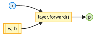
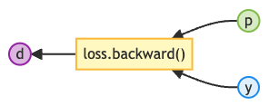
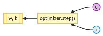
More specifically, the process of feeding one data record to the network and finally updating the model parameters once is called one iteration. Each iteration consists of three steps. For our simplest network model:

Forward propagation:

Forward propagation: the feature x goes through layer.forward() together with the parameters w and b to produce the prediction p

Figure: Forward propagation (model inference)

Backpropagation:

Backpropagation: loss.backward() computes the error term d from the prediction p and the label y

Figure: Backpropagation (gradient computation)

Parameter update:

Parameter update: optimizer.step() updates the parameters w and b from the error term d and the feature x

Figure: Parameter update

import numpy as np

Tensor¶

class Tensor:

    def __init__(self, data):
        self.data = np.array(data)
        self.grad = np.zeros_like(self.data)
        self.gradient_fn = None
        self.parents = []

    def backward(self):
        if self.gradient_fn is not None:
            self.gradient_fn()

        for p in self.parents:
            p.backward()

    def __str__(self):
        return f'Tensor({self.data})'

Dataset¶

The massive data needed for model training is called the dataset.

Each record in the dataset is called a sample. Each sample consists of two parts: the feature and the label.

A dataset is usually split into two parts:

Training set: the larger part (for example, 80%), used for model training;
Test set: the smaller part (for example, 20%), used for model evaluation.

The purpose of splitting the dataset is to hold back some new data: the test set. With new data, we can verify whether the trained network model has really learned the patterns, rather than just memorizing some of the content. It is like a final exam: the teacher does not use the exercises you have already done as the exam paper, but a new set of questions to check whether you have truly mastered what you learned.

Ming provided the weather forecasts and sales records of the past four days, which serve as our training set. The data we used before serves as the test set.

A dataset usually provides the following functions:

load (load method): loads all the data;
train (training method): switches to model training mode;
eval (test method): switches to model testing mode;
all (all samples): returns all the samples;
__len__ (number of samples): returns the number of samples;
__getitem__(index) (a single sample): returns the sample for the given index (index).

class Dataset:

    def __init__(self):
        # Load the data
        self.load()
        # Use the training set by default
        self.train()

    # Load method
    def load(self):
        # Training set
        self.train_data = ([[22.5, 72.0],
                            [31.4, 45.0],
                            [19.8, 85.0],
                            [27.6, 63.0]],
                           [[95],
                            [210],
                            [70],
                            [155]])
        # Test set
        self.test_data = ([[28.1, 58.0]],
                          [[165]])

    # Training method
    def train(self):
        self.data = self.train_data

    # Test method
    def eval(self):
        self.data = self.test_data

    # All samples
    def all(self):
        x, y = self.data
        return Tensor(x), Tensor(y)

    # Number of samples
    def __len__(self):
        x, *_ = self.data
        return len(x)

    # A single sample
    def __getitem__(self, index):
        x, y = self.data
        return Tensor(x[index]), Tensor(y[index])

Model¶

class Linear:

    def __init__(self, in_size, out_size):
        self.weight = Tensor(np.ones((out_size, in_size)) / in_size)
        self.bias = Tensor(np.zeros(out_size))

    def __call__(self, x: Tensor):
        return self.forward(x)

    def forward(self, x: Tensor):
        p = Tensor(x.data @ self.weight.data.T + self.bias.data)

        def gradient_fn():
            self.weight.grad += p.grad * x.data
            self.bias.grad += np.sum(p.grad)

        p.gradient_fn = gradient_fn
        return p

    @property
    def parameters(self):
        return [self.weight, self.bias]

Loss function (mean squared error)¶

class MSELoss:

    def __call__(self, p: Tensor, y: Tensor):
        return self.loss(p, y)

    def loss(self, p: Tensor, y: Tensor):
        mse = Tensor(np.mean(np.square(y.data - p.data)))

        def gradient_fn():
            p.grad += -2 * (y.data - p.data)

        mse.gradient_fn = gradient_fn
        mse.parents = [p]
        return mse

Optimizer (stochastic gradient descent)¶

To meet the new need for multiple iterations during model training, we upgrade the optimizer by adding a new function:

zero_grad (zeroing method): clears all the gradients before each iteration, getting ready for the next round of gradient computation.

💡 Tip: Why do we need to clear the gradients before every iteration? Look at the gradient functions of tensors such as the weights: the gradients they compute are accumulated. If we do not clear them before each iteration, the new gradients are added on top of the old gradients accumulated in previous iterations, and they keep growing.

class SGDOptimizer:

    def __init__(self, parameters, lr):
        self.parameters = parameters
        self.lr = lr

    # Zeroing method
    def zero_grad(self):
        for p in self.parameters:
            p.grad = np.zeros_like(p.data)

    def step(self):
        for p in self.parameters:
            p.data -= p.grad * self.lr

Hyperparameters¶

Learning rate¶

LEARNING_RATE = 0.00001

Modeling¶

We need to create an instance of the dataset.

dataset = Dataset()
model = Linear(2, 1)
loss_fn = MSELoss()
optimizer = SGDOptimizer(model.parameters, lr=LEARNING_RATE)

Training¶

Now our dataset has multiple training samples, so we need a loop: each time, take one sample from the dataset and complete one iteration.

Every iteration follows the same five steps, and this order will stay stable in later chapters:

Zero the gradients (zero_grad): clear the gradients computed in the previous iteration;
Forward propagation (forward): compute the prediction;
Compute the loss (loss): get the loss;
Backpropagation (backward): compute the gradients of all the nodes in the computational graph;
Update the parameters (step): adjust the parameters with the gradients.

Remember this “five-step loop”. It is the core skeleton of almost all deep learning training code.

# Iterate
for i in range(len(dataset)):
    feature, label = dataset[i]

    # Zero the gradients
    optimizer.zero_grad()
    # Forward propagation (build the computational graph)
    prediction = model(feature)
    # Compute the loss
    loss = loss_fn(prediction, label)
    # Backpropagation (compute the gradients)
    loss.backward()
    # Update the parameters
    optimizer.step()

Inference¶

After training, we switch the dataset to test mode and evaluate the training result with new data (the test set).

# Use the test set
dataset.eval()
feature, label = dataset.all()

prediction = model(feature)
print(f'prediction:\t{prediction}')

prediction:	Tensor([[67.20489976]])

Evaluation¶

loss = loss_fn(prediction, label)
print(f'loss:\t{loss}')

loss:	Tensor(9563.881631333801)

The evaluation shows that after 4 iterations the loss keeps decreasing, and the network model has improved again. But there is still a lot of room for improvement.

Exercises¶

Does the order of the training data affect the result of model training? Try shuffling the training data (for example, reversing the order), train again, and observe what changes.