We have successfully trained our first neural network model, which predicts ice cream sales from the weather forecast.
But are ice cream sales really determined directly by the weather?
In fact, the weather is not a direct factor. The weather first affects people’s behavior and preferences, such as whether they feel like going out and whether they feel like eating ice cream.
When the weather is cool: people are more willing to go out, but may not want ice cream;
When the weather is hot: people want ice cream more, but may be unwilling to go out;
When the weather is cold: people neither want to go out nor want ice cream.
From this perspective, ice cream sales are not determined directly by the weather, but jointly by people’s desire to go out and their desire to eat ice cream.
So, can we do this:
first use one model to predict these intermediate factors from the weather;
then use another model to predict ice cream sales from these intermediate factors?
Going further, can we use the output of the first model directly as the input of the second model, and connect the two models into a whole?
If so, then during training, can we pass the prediction error of the ice cream sales back to the first model through backpropagation, so that both models are trained at the same time?
The ability to learn intermediate factors automatically inside the network model is exactly what makes deep neural networks special.
Layers
A modern deep neural network consists of many layers, and each layer can be seen as a small, independent network model. In our example, we will build a two-layer network model.
A multi-layer network model has the same three core processes: forward propagation, backpropagation, and parameter update, and they run through every layer:
Forward propagation:
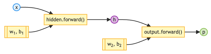
Backpropagation:
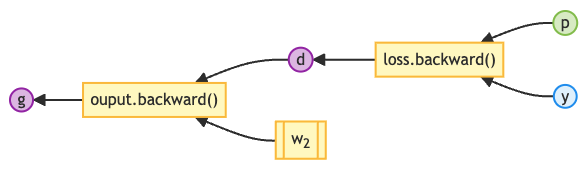
Parameter update:
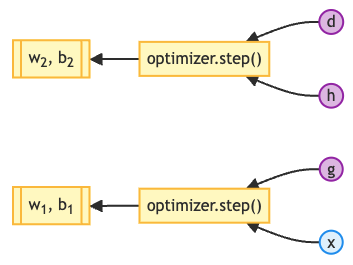
from abc import ABC, abstractmethod

import numpy as npnp.random.seed(42)💡 Tip: The function
np.random.seed()initializes the random number generator, so that every run produces the same random numbers and the results are reproducible.
Tensor
class Tensor:

    def __init__(self, data):
        self.data = np.array(data)
        self.grad = np.zeros_like(self.data)
        self.gradient_fn = None
        self.parents = set()

    def backward(self):
        if self.gradient_fn is not None:
            self.gradient_fn()

        for p in self.parents:
            p.backward()

    def __str__(self):
return f'Tensor({self.data})'Dataset
class Dataset:

    def __init__(self, batch_size=1):
        self.batch_size = batch_size
        self.load()
        self.train()

    def load(self):
        self.train_data = ([[22.5, 72.0],
                            [31.4, 45.0],
                            [19.8, 85.0],
                            [27.6, 63.0]],
                           [[95],
                            [210],
                            [70],
                            [155]])
        self.test_data = ([[28.1, 58.0]],
                          [[165]])

    def train(self):
        self.data = self.train_data

    def eval(self):
        self.data = self.test_data

    def all(self):
        x, y = self.data
        return Tensor(x), Tensor(y)

    def __len__(self):
        x, *_ = self.data
        return len(x) // self.batch_size

    def __getitem__(self, index):
        s = slice(index * self.batch_size, (index + 1) * self.batch_size)
        x, y = self.data
return Tensor(x[s]), Tensor(y[s])Model
From now on, we will build our first complex neural network model made up of several sub-networks, called a multi-layer network model.
These layers are connected to one another through a uniformly defined interface, which makes up a large, complex network model.
Abstract layer
So we first need to define a specification that all layers follow, called the abstract layer. It requires every layer to implement two things:
forward(the forward method): takes the input vector and computes the output vector. This is where each layer performs forward propagation;parameters(the parameter list): returns the parameters of this layer that need to be trained and updated. It is an empty list by default.
💡 Tip:
ABCmarks a Python abstract base class. It means that the class cannot be instantiated and can only be inherited.@abstractmethoddefines an abstract method in it, that is, a method that subclasses must implement.
class Layer(ABC):

    def __call__(self, x: Tensor):
        return self.forward(x)

    @abstractmethod
    def forward(self, x: Tensor):
        pass

    @property
    def parameters(self):
        return []
Linear layer
With the abstract layer in place, we rewrite our existing linear regression model as a linear layer. We also add two important features:
Random weight initialization
Until now we have always initialized the weights to the average value: np.ones((out_size, in_size)) / in_size. That is fine for a simple model, but in a multi-layer model, identical initial weights produce identical outputs, and therefore identical gradients, so all the outputs stay exactly the same forever. All the extra neurons are wasted. This phenomenon is called symmetry in model training.
The solution is simple: give every neuron different initial weights, so that the output and gradient of each neuron develop in different directions. We use np.random.randn to generate (different) random numbers, and then a scaling factor np.sqrt(2 / in_size) to adjust their range. This factor keeps the initial weights in a reasonable range and prevents the gradient from growing or shrinking layer after layer as it propagates through the network. This initialization method is called He initialization.
Passing the gradient to the parent nodes
The earlier simple model only had to compute the gradient of its own weights.
With multiple layers, we also have to pass the gradient to the previous layers (the parent nodes). That is, the input may no longer be a feature, but an intermediate value coming from the previous layer. So:
the gradient function must compute the gradient of the input;
the input must be added to the parent list, because the input is no longer a leaf node but an intermediate node.
💡 Tip: These two lines of code are crucial. They connect the multi-layer network model, so that backpropagation can pass through the boundaries between layers and traverse the computational graph of the whole complex network model.
class Linear(Layer):

    def __init__(self, in_size, out_size):
        self.weight = Tensor(np.random.randn(out_size, in_size) * np.sqrt(2 / in_size))
        self.bias = Tensor(np.zeros(out_size))

    def forward(self, x: Tensor):
        p = Tensor(x.data @ self.weight.data.T + self.bias.data)

        def gradient_fn():
            self.weight.grad += p.grad.T @ x.data
            self.bias.grad += np.sum(p.grad, axis=0)
            # Compute the gradient of the input
            x.grad += p.grad @ self.weight.data

        p.gradient_fn = gradient_fn
        # Add the input to the parent list
        p.parents = [x]
        return p

    @property
    def parameters(self):
        return [self.weight, self.bias]
Sequential layer
The sequential layer is our first composite layer.
A composite layer can be seen as a container of several sublayers. The sequential layer is the simplest kind: it runs each sublayer in order.
forward(the forward method): passes the input through every layer in turn, with the output of each layer being the input of the next, and the output of the last layer is the prediction;parameters(the parameter list): combines the parameter lists of all the layers into one big list and gives it to the optimizer at once, so that all the parameters are updated.
💡 Tip: The sequential layer itself inherits from the abstract layer, so it can also be a sublayer of another sequential layer (or of another composite layer). This lets us “stack blocks” to build larger network models.
class Sequential(Layer):

    def __init__(self, layers):
        self.layers = layers

    def forward(self, x: Tensor):
        # Run each sublayer in order
        for l in self.layers:
            x = l(x)
        return x

    @property
    def parameters(self):
        # Combine the parameters of all sublayers
        return [p for l in self.layers for p in l.parameters]
Loss function (mean squared error)
class MSELoss:

    def __call__(self, p: Tensor, y: Tensor):
        return self.loss(p, y)

    def loss(self, p: Tensor, y: Tensor):
        mse = Tensor(np.mean(np.square(y.data - p.data)))

        def gradient_fn():
            p.grad += -2 * (y.data - p.data) / y.data.size

        mse.gradient_fn = gradient_fn
        mse.parents = [p]
        return mse
Optimizer (stochastic gradient descent)
class SGDOptimizer:

    def __init__(self, parameters, lr):
        self.parameters = parameters
        self.lr = lr

    def zero_grad(self):
        for p in self.parameters:
            p.grad = np.zeros_like(p.data)

    def step(self):
        for p in self.parameters:
p.data -= p.grad * self.lrTrainer
class Trainer:

    def __init__(self, model, loss_fn, optimizer):
        self.model = model
        self.loss_fn = loss_fn
        self.optimizer = optimizer

    def train(self, dataset, epochs):
        dataset.train()

        for epoch in range(epochs):
            for i in range(len(dataset)):
                feature, label = dataset[i]

                self.optimizer.zero_grad()
                prediction = self.model(feature)
                loss = self.loss_fn(prediction, label)
                loss.backward()
                self.optimizer.step()

    def test(self, dataset):
        dataset.eval()

        feature, label = dataset.all()
        prediction = self.model(feature)
        loss = self.loss_fn(prediction, label)
return prediction, lossLEARNING_RATE = 0.00001Batch size
BATCH_SIZE = 2Number of epochs
EPOCHS = 1000Modeling
Now we use a sequential layer to chain two linear layers into a two-layer network model:
The first layer,
Linear(2, 4): the input is 2 features[temperature, humidity]and the output is 4 intermediate values. These 4 intermediate values correspond to the desire to go out and the desire to eat ice cream that we imagined at the beginning, except that we give the model more freedom and let it find the real relationships in the data by itself during training;The second layer,
Linear(4, 1): the input is the 4 intermediate values output by the first layer, and the output is 1 prediction (the ice cream sales).
The 4 neurons of the first layer do not produce the output (the prediction) directly. This layer is also called the hidden layer. It is also where the network model shows its intelligence: it can capture the deep relationships in the data on its own.
The second layer, that is, the last layer, is called the output layer.
dataset = Dataset(BATCH_SIZE)
model = Sequential([
    # Hidden layer
    Linear(2, 4),
    # Output layer
    Linear(4, 1),
])
loss_fn = MSELoss()
optimizer = SGDOptimizer(model.parameters, lr=LEARNING_RATE)
trainer = Trainer(model, loss_fn, optimizer)Training
trainer.train(dataset, EPOCHS)Evaluation
prediction, loss = trainer.test(dataset)
print(f'prediction:\t{prediction}\nloss:\t{loss}')
prediction: Tensor([[166.52357679]])
loss: Tensor(2.321286244423445)
In practice, the two-layer network model works. But compared with the single-layer model, there is no obvious difference, and the loss is even slightly worse.
This is not surprising. So far, we have only stacked two layers of linear regression. Mathematically, two layers of linear regression are still linear. To make a multi-layer network model really useful, we are missing one last piece of the puzzle: introducing nonlinearity.
Exercises
Change the number of neurons in the hidden layer (for example, to 2 or 8) and observe how the training result changes.
Can we add more hidden layers (for example, 2 or 3)? Try to implement it.