In the first ten chapters, we built a basic neural network training framework from scratch and used it to implement a two-layer network model that predicts ice cream sales. The same method can solve a large number of regression and classification problems.
⚠️ Note: In classification problems, an activation function in the output layer will come into play.
In real life, there is another large and more complex class of problems: time series.
The defining feature of such data is a clear order. We cannot look only at the current set of data; we also need to refer to all the data before it. For stock prices, for example, we cannot look only at today’s price. We must also consider how prices have changed over a long period.
Among all time series data, the one closest to human intelligence, and also the most complex, is language. From this part on, we will extend our neural network training framework to process text.
The first problem we face is how to digitize text. A neural network can only process numbers, so we need a way to convert text into numbers.
Index encoding
The most direct method is to line up all the characters (or words) and give each of them a number in turn. This is called index encoding.
For example, take the 26 English letters. The first three letters are A, B, and C, so their index encodings are 0, 1, and 2, while the index encodings of X, Y, and Z are 23, 24, and 25.
But index encoding is still not suitable for neural networks, because it may lead the model to believe that B, represented by 1, is greater than A, represented by 0.
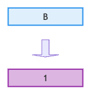
One-hot encoding
A better solution is one-hot encoding. The core idea is very intuitive. Again take the 26 English letters: map each letter to a vector whose length equals the total number of letters (26). In this vector, exactly one position is 1 (the position given by the index encoding), and all the other positions are 0.
For example, the one-hot encoding of A is [1, 0, 0 ... 0], that of B is [0, 1, 0 ... 0], and that of Z is [0, 0, 0 ... 1]. In this way, the encodings of all letters are mathematically equidistant, and no letter is more special than any other.

How, then, do we represent a word, or even a whole sentence?
Bag of words
A simple but effective way is the bag of words: add up the one-hot encoding vectors of all the letters in a word, or even in a whole sentence, to get a vector sum. This tells us which characters appear in the word or sentence, and how many times each one appears.
For example, the bag of words of BED is [0, 1, 0, 1, 1, 0 ... 0], and that of BEE is [0, 1, 0, 0, 2, 0 ... 0].
💡 Tip: The bag-of-words model is simple and clear, but it has an obvious drawback: it loses the order of the characters. For example,
EATandTEAhave exactly the same bag-of-words representation, so they cannot be told apart.

from abc import ABC, abstractmethod
from pathlib import Path

import numpy as np
import requestsnp.random.seed(42)Tensor
class Tensor:

    def __init__(self, data):
        self.data = np.array(data)
        self.grad = np.zeros_like(self.data)
        self.gradient_fn = None
        self.parents = set()

    def backward(self):
        if self.gradient_fn is not None:
            self.gradient_fn()

        for p in self.parents:
            p.backward()

    def __str__(self):
return f'Tensor({self.data})'Dataset
We remove the concrete data from the dataset of the first ten chapters and turn it into an abstract dataset class with the basic functions.
Abstract class
The abstract class keeps all the basic functions that every dataset must provide:
load(load method): loads the data. This is an abstract method interface;train(training method): provides the training set data;eval(test method): provides the test set data;all(all samples): reads all the samples;__len__(number of samples): returns the number of samples;__getitem__(a single sample): reads a sample by index.
class Dataset(ABC):

    def __init__(self, batch_size=1):
        self.batch_size = batch_size
        self.load()
        self.train()

    @abstractmethod
    def load(self):
        pass

    def train(self):
        self.data = self.train_data

    def eval(self):
        self.data = self.test_data

    def all(self):
        x, y = self.data
        return Tensor(x), Tensor(y)

    def __len__(self):
        x, *_ = self.data
        return len(x) // self.batch_size

    def __getitem__(self, index):
        s = slice(index * self.batch_size, (index + 1) * self.batch_size)
        x, y = self.data
        return Tensor(x[s]), Tensor(y[s])
Character-encoding dataset
From this part on, we will focus on plain text data.
Tokenization
When processing plain text, the first problem we meet is usually how to divide the data into units. This is called tokenization. Common methods are:
Word level: the units are semantically complete and match the habits of language. But the vocabulary is usually huge. An English vocabulary, for example, can reach tens of thousands or even more than a hundred thousand words. It also cannot handle out-of-vocabulary words well, such as new words and rare words.
Character level: the vocabulary is very small. An English vocabulary, for example, has only a few dozen characters, and there is no problem with new or rare words. But it loses the semantics of words, and the data sequences become very long after tokenization.
Subword level: this is the mainstream approach in modern large language models. It sits between words and characters and tries to balance vocabulary size against semantic expressiveness. It keeps common words intact and splits rare words into smaller units (subwords). The most commonly used algorithm is byte pair encoding (BPE): starting from characters, it counts frequencies and gradually merges the character pairs that occur together most often.
We will tokenize by character. This is a common choice for building a tiny LLM. It suits tiny datasets and has low computing requirements.
Preprocessing
The dataset is a large piece of complete text. We will use the selected Shakespeare plays (tinyshakespeare).
After loading the text, we first need to preprocess it:
Build the vocabulary: collect all the letters, digits, punctuation marks, and other special characters used in the text to form the vocabulary;
Index encoding: give every character in the vocabulary an index encoding.
After preprocessing, the dataset will contain:
vocab(vocabulary): the collection of all the characters used;index tables:
stoi(forward index table): the lookup table from characters to index encodings;itos(reverse index table): the lookup table from index encodings to characters;
tokens(token table): the whole text converted into index encodings. This is the data the model can process.
The character-encoding dataset also provides two additional functions:
encode(encoding method): returns the index encoding of a text;decode(decoding method): converts index encodings back into text.
Features and labels
The preprocessed token table is finally split into features and labels. Depending on the task, there are several ways to split it:
Text classification tasks: for example, spam classification and customer feedback analysis.
Feature: the token sequence of an email, or of a piece of customer feedback;
Label: the category (for example,
1for a spam email, or a customer rating from1to5);
Sequence labeling tasks: for example, part-of-speech tagging and entity recognition.
Feature: a token sequence (for example,
[he, is, young]);Label: the sequence of labels matching the part of speech of each token (for example,
[N, V, J]).
Self-supervised training: for example, a GPT model predicting the next word.
Feature: a token sequence cut from the training text;
Label: the next token after the feature token sequence.
Text classification and sequence labeling tasks both need extra data (such as customer ratings) or manual annotation. Large language models usually use self-supervised training, which is also what we will use.
Example
Let’s see how a language model generates text. Suppose our training text is this passage:
BUCKINGHAM: My lord, I claim your gift, ...During training, each time we cut several characters (for example, 8) from the text as the feature. The first training sample is BUCKINGH, and what we want to predict is the 9th character: A.
We combine the one-hot encodings of the feature into a bag of words, which gives:
[0, 1, 1, 0, 0, 0, 1, 1, 1, 0, 1, 0, 0, 1, 0, 0, 0, 0, 0, 0, 1, 0, 0, 0, 0, 0, 0 ...]And the one-hot encoding of the label is:
[1, 0, 0, 0, 0, 0, 0, 0, 0, 0, 0, 0, 0, 0, 0, 0, 0, 0, 0, 0, 0, 0, 0, 0, 0, 0, 0 ...]So the essence of a language model is a multi-class classification model that predicts one encoding array from another.
For the second training sample, we shift forward by one or more characters and cut the data again. If we shift by two characters, the feature is now CKINGHAM and the label is :.
Their encodings (the feature bag of words and the label one-hot encoding) are:
[1, 0, 1, 0, 0, 0, 1, 1, 1, 0, 1, 0, 1, 1, 0, 0, 0, 0, 0, 0, 0, 0, 0, 0, 0, 0, 0 ...]
[0, 0, 0, 0, 0, 0, 0, 0, 0, 0, 0, 0, 0, 0, 0, 0, 0, 0, 0, 0, 0, 0, 0, 0, 0, 0, 1 ...]
After that, we keep shifting forward and cutting new training data until the end of the training text, which completes one epoch.
Initialization parameters
The character-encoding dataset needs three additional initialization parameters:
context_size(context size): how many tokens to cut as the feature each time;stride(context stride): how many tokens to skip before cutting the next label. We use half of the context size as the default;split(training/test split ratio): the fraction of the text used as the training set. The remaining text is used as the test set.
class CharDataset(Dataset):

    def __init__(self, filename, batch_size=1, context_size=64, stride=None, split=0.9):
        self.filename = filename
        self.context_size = context_size
        self.stride = stride if stride is not None else context_size // 2
        self.split = split
        super().__init__(batch_size)

    def load(self):
        with open(self.filename, encoding="utf-8") as f:
            text = f.read()

        # Vocabulary
        self.vocab = sorted(set(text))
        self.vocab_size = len(self.vocab)
        # Index tables
        self.stoi = {ch: i for i, ch in enumerate(self.vocab)}
        self.itos = {i: ch for i, ch in enumerate(self.vocab)}
        # Token table
        self.tokens = self.encode(text)

        # Split into training and test sets
        split = int(len(self.tokens) * self.split)
        self.train_data = self._pack(self.tokens[:split])
        self.test_data = self._pack(self.tokens[split:])

    # Cut the samples
    def _pack(self, tokens):
        onehot = np.eye(self.vocab_size)
        x, y = [], []
        for i in range(0, len(tokens) - self.context_size - 1, self.stride):
            # Feature: bag of words of one-hot encodings
            x.append(onehot[tokens[i: i + self.context_size]].sum(axis=0))
            # Label: one-hot encoding
            y.append(onehot[tokens[i + self.context_size]])
        return x, y

    # Encoding method
    def encode(self, symbols):
        return [self.stoi[s] for s in symbols]

    # Decoding method
    def decode(self, tokens):
return "".join(self.itos[t] for t in tokens)class Layer(ABC):
def __call__(self, x: Tensor):
return self.forward(x)
@abstractmethod
def forward(self, x: Tensor):
pass
@property
def parameters(self):
return []Linear layer
class Linear(Layer):

    def __init__(self, in_size, out_size):
        self.weight = Tensor(np.random.randn(out_size, in_size) * np.sqrt(2 / in_size))
        self.bias = Tensor(np.zeros(out_size))

    def forward(self, x: Tensor):
        p = Tensor(x.data @ self.weight.data.T + self.bias.data)

        def gradient_fn():
            self.weight.grad += p.grad.T @ x.data
            self.bias.grad += np.sum(p.grad, axis=0)
            x.grad += p.grad @ self.weight.data

        p.gradient_fn = gradient_fn
        p.parents = [x]
        return p

    @property
    def parameters(self):
        return [self.weight, self.bias]
Sequential layer
class Sequential(Layer):

    def __init__(self, layers):
        self.layers = layers

    def forward(self, x: Tensor):
        for l in self.layers:
            x = l(x)
        return x

    @property
    def parameters(self):
        return [p for l in self.layers for p in l.parameters]
Activation functions
We keep only the two activation functions we will use: ReLU and Softmax.
Rectified linear unit (ReLU)
class ReLU(Layer):

    def forward(self, x: Tensor):
        a = Tensor(np.maximum(0, x.data))

        def gradient_fn():
            x.grad += a.grad * (a.data > 0)

        a.gradient_fn = gradient_fn
        a.parents = [x]
return aSoftmax
class Softmax(Layer):

    def __init__(self, axis=-1):
        super().__init__()
        self.axis = axis

    def forward(self, x: Tensor):
        exp = np.exp(x.data - np.max(x.data, axis=self.axis, keepdims=True))
        a = Tensor(exp / np.sum(exp, axis=self.axis, keepdims=True))

        def gradient_fn():
            grad = np.sum(a.data * a.grad, axis=self.axis, keepdims=True)
            x.grad += a.data * (a.grad - grad)

        a.gradient_fn = gradient_fn
        a.parents = [x]
        return a
Loss function (mean squared error)
class MSELoss:

    def __call__(self, p: Tensor, y: Tensor):
        return self.loss(p, y)

    def loss(self, p: Tensor, y: Tensor):
        mse = Tensor(np.mean(np.square(y.data - p.data)))

        def gradient_fn():
            p.grad += -2 * (y.data - p.data) / y.data.size

        mse.gradient_fn = gradient_fn
        mse.parents = [p]
        return mse
Optimizer (stochastic gradient descent)
class SGDOptimizer:

    def __init__(self, parameters, lr):
        self.parameters = parameters
        self.lr = lr

    def zero_grad(self):
        for p in self.parameters:
            p.grad = np.zeros_like(p.data)

    def step(self):
        for p in self.parameters:
p.data -= p.grad * self.lrTrainer
For text generation models, we add a new generation method generate to the trainer. It takes a prompt and lets the model continue the text automatically.
The logic of the generation method is basically the same as that of the test method. The difference is that it treats the prompt as the dataset and appends each newly generated character to the prompt one by one, so that the dataset keeps growing and the inference keeps going.
For example, we use ROMEO: as the prompt. The model generates the next character D; in the next round, the prompt is extended to ROMEO:D, and the model generates the next character e from it; the prompt is extended again to ROMEO:De, and the model keeps generating new characters from the extended prompt.
class Trainer:

    def __init__(self, model, loss_fn, optimizer):
        self.model = model
        self.loss_fn = loss_fn
        self.optimizer = optimizer

    def train(self, dataset, epochs):
        dataset.train()

        for epoch in range(epochs):
            for i in range(len(dataset)):
                feature, label = dataset[i]

                self.optimizer.zero_grad()
                prediction = self.model(feature)
                loss = self.loss_fn(prediction, label)
                loss.backward()
                self.optimizer.step()

    def test(self, dataset):
        dataset.eval()

        feature, label = dataset.all()
        prediction = self.model(feature)
        loss = self.loss_fn(prediction, label)
        return prediction, loss

    # Generation method
    def generate(self, dataset, prompt, steps=256):
        tokens = dataset.encode(prompt)
        onehot = np.eye(dataset.vocab_size)

        for _ in range(steps):
            # Inference
            window = tokens[-dataset.context_size:]
            feature = Tensor([onehot[window].sum(axis=0)])
            prediction = self.model(feature)

            # Sampling
            probs = prediction.data[0] / np.sum(prediction.data[0])
            token = np.random.choice(len(probs), p=probs)
            # Append the new token to the prompt
            tokens.append(token)

return dataset.decode(tokens)LEARNING_RATE = 0.01Batch size
BATCH_SIZE = 4Number of epochs
EPOCHS = 10Context size
This is a new hyperparameter. The context size defines the length of data cut from the token table each time, that is, how long a piece of text we use in each training step to predict the next letter.
A longer context size provides more information for inference and improves its accuracy. But it also increases the computing requirements of training and inference, so it has to be weighed carefully. The earliest large language models usually used a context size in the range of 1024 to 4096. Today’s top large language models can already exceed 1M.
CONTEXT_SIZE = 32Data preparation
Before training, there is one last preparation step: downloading the training data. We will use a dataset that is very popular in teaching, the tiny Shakespeare plays (tinyshakespeare), which can be downloaded from the URL below.
DATA_FILE = "../../../../data/tinyshakespeare.txt"

file = Path(DATA_FILE)
if not file.exists():
    file.parent.mkdir(parents=True, exist_ok=True)
    url = "https://raw.githubusercontent.com/karpathy/char-rnn/master/data/tinyshakespeare/input.txt"
    response = requests.get(url)
    response.raise_for_status()
file.write_text(response.text)Modeling
We will build a two-layer network model:
Linear(vocab_size, vocab_size * 2): the input of the first layer (the hidden layer) is the bag of words of a group of tokens (as many as the context size), so its size is the size of the dataset’s vocabulary (vocab). We make the output size of the first layer twice its input size;ReLU(): after the first layer, we use ReLU as the hidden layer activation function, which is the standard practice;Linear(vocab_size * 2, vocab_size): the input of the second layer (the output layer) is the output of the first layer. The output of the second layer is the prediction, that is, the one-hot encoding of the next letter, so its size is also the size of the dataset’s vocabulary (vocab);Softmax(): after the second layer, we use Softmax as the output layer activation function. This is because the model’s output is really a multi-class classification: choosing the character with the highest probability from the dataset’s vocabulary.
The input data (the feature) of the model has the shape (batch size, vocabulary size); the output of the hidden layer has the shape (batch size, vocabulary size * 2); and the output (the prediction) of the output layer returns to (batch size, vocabulary size).
dataset = CharDataset(DATA_FILE, BATCH_SIZE, CONTEXT_SIZE)
model = Sequential([
    # Hidden layer
    Linear(dataset.vocab_size, dataset.vocab_size * 2),
    # Hidden layer activation function
    ReLU(),
    # Output layer
    Linear(dataset.vocab_size * 2, dataset.vocab_size),
    # Output layer activation function
    Softmax()
])
loss_fn = MSELoss()
optimizer = SGDOptimizer(model.parameters, lr=LEARNING_RATE)
trainer = Trainer(model, loss_fn, optimizer)Training
trainer.train(dataset, EPOCHS)Evaluation
prediction, loss = trainer.test(dataset)
print(f'prediction:\t{prediction.data.shape}\nloss:\t{loss}')
prediction: (6970, 65)
loss: Tensor(0.014733022893551677)
Inference
Finally, we use the trained model to generate text for the first time. The prompt is ROMEO:.
print(trainer.generate(dataset, prompt="ROMEO:"))ROMEO:Et
KiQ $fxaXKB
BS3 itwg
k inlxjh?s,sG o
o,sooH r Tna t
y! i ot
se3Au ti isrhsBtsiqhifTeIaJ LoMl;Y.:ihGbr. k yheaf!tf:e'
ffe&d echsrwwjtsh oKj Jht spMW
e-CshoBorowpoo a
3wKxo.f xo
so
oo o
c
to O o
oto-UnoooUt oo oto
!V xoLupAU:xctLs xtTomtLZrlWo lANece
We hoped the model would continue a piece of Romeo’s dialogue. As expected, we got an output that is almost gibberish.
In this chapter, we successfully implemented a language model that learns from text and produces text. In the next few chapters, we will gradually extend the model to improve its output.
Exercises
The context size is arguably the most important hyperparameter of a language model. Try changing it to different values (for example, reduce it to
16or increase it to64) and see how the generated text differs after training.