Recurrent neural network - From Neuron to GPT

So far, our simple text generation model still has two bottlenecks on the road to real language understanding:

It cannot understand word order: “the mouse loves rice” and “rice loves the mouse” produce the same context feature. The important information of the order in which words appear is lost.
It lacks long-range memory: the model’s view is limited to a narrow context size. For text beyond that range, the model cannot build any association between the meanings. Take this lyric: “I love you like a mouse loves rice”. With a context size of 5, the model cannot learn the association between “I love you” and “a mouse loves rice”.

How to give a machine “long-term memory” is not a new problem.

In 1990, the linguist Elman proposed the Simple RNN. Elman fed the hidden state back into the next moment, which became the standard paradigm of the modern recurrent neural network (RNN): the model looks not only at the current input, but also at its own past.

The hidden state is the state of the input data inside the network after layer upon layer of transformation, just before it enters the final output layer. It holds a summary of everything the network has learned up to this moment, which is what we call temporal memory.

Looking back at our word vector model, it has three layers: the embedding layer, the hidden layer, and the output layer. The output of the hidden layer (after the activation function) is the hidden state.

Simply put, a recurrent neural network calls the process of reading one character a time step, and connects the hidden state of the previous time step, taken just before the output layer, to the word vector built by the embedding layer in the current time step. A time step then consists of four steps:

the embedding layer does the first round of learning on the input data and produces a word vector;
the word vector is connected with the hidden state of the previous time step;
the word vector, now carrying temporal memory, is learned from further, producing the hidden state of the current time step;
the output layer produces the prediction.

The final output has two parts, the prediction and the hidden state. The prediction is used by the loss function to start the gradient computation and backpropagation, and the hidden state takes part in the next time step.

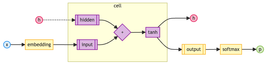
Recurrent neural network: the input feature x and the hidden state h of the previous time step together produce the new hidden state h′, from which the prediction p′ is obtained

Figure: Recurrent neural network

Where:

$x$ : the (input) feature;
$h$ : the hidden state (of the previous time step);
$h^{\prime}$ : the (output) hidden state;
$p^{\prime}$ : the (output) prediction.

from abc import ABC, abstractmethod

import numpy as np

np.random.seed(42)

Tensor¶

Backward method¶

The backward method of a tensor is the main carrier of backpropagation: in it, we traverse all the parent nodes in the computational graph and compute their gradients.

So far we have used a very simple recursive traversal. It works when all the nodes of the graph form a line or a tree, where each node is visited only once. A recurrent neural network breaks exactly this assumption. In an RNN, the hidden state $h$ has to be sent to the output layer to produce a prediction and also passed to the next time step to be updated further, so the same node is reached by two paths and visited once on each; and the same computation is called dozens of times. As a result, the same node in the computational graph is visited several times, and its gradient is computed repeatedly.

The fix is to switch to a topological sort: first arrange all the nodes of the graph in dependency order, so that every node comes after all of its parent nodes. Then, starting from the end of this node sequence (the loss tensor), we visit each node in reverse order and compute its gradient. Each node is visited once and only once, so the gradient computation neither repeats nor misses anything.

Addition¶

An important step of an RNN is adding the hidden state $h$ of the previous time step to the new feature embedding vector. This is not a simple addition of two vectors: like the embedding layer and the mean pooling layer, it has to build the computational graph in forward propagation and compute the gradients in backpropagation.

Our solution is to extend the addition operation of the tensor: while adding, we also implement the gradient function gradient_fn and the parent list parents of the resulting tensor.

class Tensor:

    def __init__(self, data):
        self.data = np.array(data)
        self.grad = np.zeros_like(self.data)
        self.gradient_fn = None
        self.parents = set()

    def backward(self):
        # Topological order
        topo = []
        # Visited nodes
        visited = set()
        # Stack (node, whether its parents have been expanded)
        stack = [(self, False)]

        # Build the topological order
        while stack:
            node, expanded = stack.pop()
            if node in visited:
                continue

            if expanded:
                visited.add(node)
                topo.append(node)
            else:
                stack.append((node, True))
                for p in node.parents:
                    if p not in visited:
                        stack.append((p, False))

        # The initial gradient of the starting node is 1
        self.grad = np.ones_like(self.data)
        # Visit in reverse order and backpropagate
        for t in reversed(topo):
            if t.gradient_fn is not None:
                t.gradient_fn()

        # After backpropagation, clear the computational graph
        for t in topo:
            t.gradient_fn = lambda: None
            t.parents = set()

    # Tensor addition
    def __add__(self, other):
        p = Tensor(self.data + other.data)

        def gradient_fn():
            self.grad += p.grad
            other.grad += p.grad

        p.gradient_fn = gradient_fn
        p.parents = [self, other]
        return p

    def __str__(self):
        return f'Tensor({self.data})'

Dataset¶

Abstract class¶

class Dataset(ABC):

    def __init__(self, batch_size=1):
        self.batch_size = batch_size
        self.load()
        self.train()

    @abstractmethod
    def load(self):
        pass

    def train(self):
        self.data = self.train_data

    def eval(self):
        self.data = self.test_data

    def all(self):
        x, y = self.data
        return Tensor(x), Tensor(y)

    def __len__(self):
        x, *_ = self.data
        return len(x) // self.batch_size

    def __getitem__(self, index):
        s = slice(index * self.batch_size, (index + 1) * self.batch_size)
        x, y = self.data
        return Tensor(x[s]), Tensor(y[s])

Character-encoding dataset¶

In the previous chapters, we always used the one-hot encoding of the next character as the label of a sample.

An RNN, however, processes a sample one character at a time. For example, with a context size of 32, each sample is 32 characters. Starting from the first character, the RNN makes 32 predictions in turn, each time carrying the hidden state of the previous step. In total it predicts 32 characters, which correspond exactly to the 32 characters shifted by one position.

So in an RNN model we will use:

$x$ (feature): tokens[i: i + self.context_size];
$y$ (label): tokens[i + 1: i + self.context_size + 1].

That is, if the feature is the characters at positions 1 to 32 of the text, the label is the characters at positions 2 to 33, which correspond to the results of the 32 predictions of the RNN.

class CharDataset(Dataset):

    def __init__(self, filename, batch_size=1, context_size=64, stride=None, split=0.9):
        self.filename = filename
        self.context_size = context_size
        self.stride = stride if stride is not None else context_size // 2
        self.split = split
        super().__init__(batch_size)

    def load(self):
        with open(self.filename, encoding="utf-8") as f:
            text = f.read()

        self.vocab = sorted(set(text))
        self.vocab_size = len(self.vocab)
        self.stoi = {ch: i for i, ch in enumerate(self.vocab)}
        self.itos = {i: ch for i, ch in enumerate(self.vocab)}
        self.tokens = self.encode(text)

        split = int(len(self.tokens) * self.split)
        self.train_data = self._pack(self.tokens[:split])
        self.test_data = self._pack(self.tokens[split:])

    def _pack(self, tokens):
        x, y = [], []
        for i in range(0, len(tokens) - self.context_size - 1, self.stride):
            # Feature: array of index encodings
            x.append(tokens[i: i + self.context_size])
            # Label: array of index encodings (shifted by 1)
            y.append(tokens[i + 1: i + self.context_size + 1])
        return x, y

    def encode(self, symbols):
        return [self.stoi[s] for s in symbols]

    def decode(self, tokens):
        return "".join(self.itos[t] for t in tokens)

Model¶

Abstract layer¶

class Layer(ABC):

    def __call__(self, *args):
        return self.forward(*args)

    @abstractmethod
    def forward(self, *args):
        pass

    @property
    def parameters(self):
        return []

Linear layer¶

class Linear(Layer):

    def __init__(self, in_size, out_size):
        self.weight = Tensor(np.random.randn(out_size, in_size) * np.sqrt(2 / in_size))
        self.bias = Tensor(np.zeros(out_size))

    def forward(self, x: Tensor):
        p = Tensor(x.data @ self.weight.data.T + self.bias.data)

        def gradient_fn():
            self.weight.grad += p.grad.T @ x.data
            self.bias.grad += np.sum(p.grad, axis=0)
            x.grad += p.grad @ self.weight.data

        p.gradient_fn = gradient_fn
        p.parents = [x]
        return p

    @property
    def parameters(self):
        return [self.weight, self.bias]

Composite layer¶

We abstract the composite layer out of the sequential layer, keeping only the function of a container for sublayers. The composite layer will be the base layer of the more complex network layers to come.

class Composite(Layer, ABC):

    def __init__(self, layers):
        super().__init__()
        self.layers = list(layers)

    @property
    def parameters(self):
        return [p for l in self.layers for p in l.parameters]

Sequential layer¶

The sequential layer now inherits from the composite layer, with the same function.

class Sequential(Composite):

    def forward(self, x: Tensor):
        for l in self.layers:
            x = l(x)
        return x

Embedding layer¶

class Embedding(Layer):

    def __init__(self, vocab_size, embedding_size, std=0.02):
        super().__init__()
        self.weight = Tensor(np.random.randn(vocab_size, embedding_size) * std)

    def forward(self, x: Tensor):
        p = Tensor(self.weight.data[x.data])

        def gradient_fn():
            np.add.at(self.weight.grad, x.data, p.grad)

        p.gradient_fn = gradient_fn
        p.parents = [self.weight]
        return p

    @property
    def parameters(self):
        return [self.weight]

Activation functions¶

Rectified linear unit (ReLU)¶

class ReLU(Layer):

    def forward(self, x: Tensor):
        a = Tensor(np.maximum(0, x.data))

        def gradient_fn():
            x.grad += a.grad * (a.data > 0)

        a.gradient_fn = gradient_fn
        a.parents = [x]
        return a

Hyperbolic tangent (Tanh)¶

class Tanh(Layer):

    def forward(self, x: Tensor):
        a = Tensor(np.tanh(x.data))

        def gradient_fn():
            x.grad += a.grad * (1 - a.data ** 2)

        a.gradient_fn = gradient_fn
        a.parents = [x]
        return a

Loss functions¶

Abstract class¶

class Loss(ABC):

    def __call__(self, p: Tensor, y: Tensor):
        return self.loss(p, y)

    @abstractmethod
    def loss(self, p: Tensor, y: Tensor):
        pass

Cross-entropy loss function¶

The dataset no longer returns one-hot encodings as labels, but sequences of index encodings in the same format as the feature.

We therefore upgrade the cross-entropy loss function. By checking the format of the label, it supports both kinds of datasets: one-hot encodings and sequences of index encodings.

class CELoss(Loss):

    def loss(self, p: Tensor, y: Tensor):
        exp = np.exp(p.data - np.max(p.data, axis=-1, keepdims=True))
        softmax = exp / np.sum(exp, axis=-1, keepdims=True)

        if y.data.ndim == softmax.ndim:
            labels = y.data
        else:
            labels = np.zeros_like(softmax)
            rows = np.arange(y.data.size)
            labels[rows, y.data] = 1

        log = np.log(np.clip(softmax, 1e-10, 1.0))
        ce = Tensor(-np.mean(np.sum(labels * log, axis=-1)))

        def gradient_fn():
            p.grad += (softmax - labels) / labels.shape[0]

        ce.gradient_fn = gradient_fn
        ce.parents = [p]
        return ce

Optimizer (stochastic gradient descent)¶

class SGDOptimizer:

    def __init__(self, parameters, lr):
        self.parameters = parameters
        self.lr = lr

    def zero_grad(self):
        for p in self.parameters:
            p.grad = np.zeros_like(p.data)

    def step(self):
        for p in self.parameters:
            p.data -= p.grad * self.lr

Recurrent neural network¶

Recurrent cell¶

The core of an RNN is the recurrent cell (Cell). It does only one thing: it fuses the character just read, $x_t$ , and the earlier memory, $h_{t-1}$ , into the new memory $h_t$ .

It has three sublayers inside:

input (input linear layer): processes the character just read, $x_t$ ;
hidden (hidden state linear layer): processes the earlier memory $h_{t-1}$ ;
tanh (activation function): squeezes the sum of the two above into $(-1, 1)$ , giving the new memory $h_t$ .

As a formula:

h_t = \tanh(W_{in} \, x_t + W_{hidden} \, h_{t-1} + b)

(1)

Where:

$h_{t-1}$ : the memory of the previous time step;
$h_t$ : the updated memory (of the current time step).

In the code, each of the two linear layers has its own bias, and $b$ in the formula is their sum.

The memory is passed on in this way, one character after another, which is where the name “recurrent” comes from.

class Cell(Composite):

    def __init__(self, in_size, out_size):
        # Input linear layer
        self.input = Linear(in_size, out_size)
        # Hidden state linear layer
        self.hidden = Linear(out_size, out_size)
        # Activation function
        self.tanh = Tanh()

        super().__init__([self.input,
                          self.hidden,
                          self.tanh])

    # Inference method (forward propagation)
    def forward(self, x: Tensor, h: Tensor):
        p = self.input(x)
        h = self.hidden(h)
        return self.tanh(p + h)

RNN model¶

Applying the recurrent cell to a complete neural network gives us the RNN. It processes a complete feature (a sequence of characters) as follows:

embedding: each character is converted into an embedding vector by the embedding layer;
cell: the embedding vector is fused with the earlier memory (the hidden state of the previous step) to give the new memory (the hidden state of this step);
output: the new memory goes through the output layer to give the predicted probabilities of the next character.

The for loop in the inference method forward feeds the character sequence of the feature, one character at a time, into the same recurrent cell cell, and passes the new memory on to the next time step. In this way, every time step trains the same set of recurrent cell parameters.

💡 Tip: So the training of an RNN has three nested loops: epochs, iterations, and time steps. This is also why it is not efficient.

Backpropagation through time¶

This structure, which shares the same cell and unrolls along the time steps, also makes the gradient flow back along the time steps all the way to the very beginning during backpropagation. This is called backpropagation through time (BPTT).

The gradient computation has to pass through dozens or even hundreds of time steps, which easily causes vanishing or exploding gradients. For this reason, RNN training can also use a technique called truncated BPTT: instead of letting the gradient pass through the whole sequence, the sequence is divided into shorter time segments, and backpropagation is carried out only within a limited number of time steps. This reduces the computation and memory cost, but it also means the model cannot directly learn dependencies over longer distances through backpropagation.

Vanishing and exploding gradients are one of the main reasons why RNNs find it hard to learn long-term dependencies. Even truncated BPTT cannot solve this problem at its root. This is also one of the reasons why improved RNNs such as LSTM and GRU, and architectures such as the Transformer, were developed afterwards.

class RNN(Composite):

    def __init__(self, vocab_size, embedding_size):
        self.embedding_size = embedding_size

        # Embedding layer
        self.embedding = Embedding(vocab_size, embedding_size)
        # Recurrent cell
        self.cell = Cell(embedding_size, embedding_size * 2)
        # Output layer
        self.output = Linear(embedding_size * 2, vocab_size)

        super().__init__([self.embedding,
                          self.cell,
                          self.output])

    # Step method
    def step(self, token: Tensor, h: Tensor):
        p = self.embedding(token)
        h = self.cell(p, h)
        return self.output(h), h

    # Inference method (forward propagation)
    def forward(self, x: Tensor, h: Tensor = None):
        batch_size, sequence_len = x.data.shape
        if h is None:
            h = Tensor(np.zeros((batch_size, self.embedding_size * 2)))

        ps = []
        # Unroll along the time steps and step through the tokens one by one
        for s in range(sequence_len):
            p, h = self.step(Tensor(x.data[:, s]), h)
            ps.append(p)

        return ps, h

Trainer¶

Abstract class¶

class Trainer(ABC):

    def __init__(self, model, loss_fn, optimizer):
        self.model = model
        self.loss_fn = loss_fn
        self.optimizer = optimizer

    @abstractmethod
    def train(self, dataset, epochs):
        pass

    @abstractmethod
    def test(self, dataset):
        pass

RNN trainer¶

Training method train: training an RNN along the time steps is slightly different from the earlier multi-layer networks. The model returns a series of predictions at once (one per time step) instead of a single prediction. So we add up the losses of all the time steps of one inference and then do a single backpropagation.

Here we make use of the addition __add__ that we added to the tensor:

loss += self.loss_fn(...)

While accumulating the loss of each time step, this also chains the computational graphs of the time steps together. With a single backpropagation, the gradient follows the computational graph through every time step and flows back to every parameter.

Generation method generate: the generation method also processes one character at a time:

First let the model process the prompt prompt token by token, updating the memory;
Predict the next character from the current memory, and update the memory again;
Repeat step 2, and chain the prediction of each step into the final output text.

class RNNTrainer(Trainer):

    def train(self, dataset, epochs):
        # Training set
        dataset.train()

        for epoch in range(epochs):
            for i in range(len(dataset)):
                feature, label = dataset[i]

                # Zero the gradients
                self.optimizer.zero_grad()
                # Forward propagation
                prediction, _ = self.model(feature)
                # Compute the loss
                loss = Tensor(0.0)
                # Accumulate the loss over the time steps
                for t in range(len(prediction)):
                    loss += self.loss_fn(prediction[t], Tensor(label.data[:, t]))
                # Backpropagation (gradients propagate along the time steps, BPTT)
                loss.backward()
                # Update the parameters
                self.optimizer.step()

    def test(self, dataset):
        # Test set
        dataset.eval()

        feature, label = dataset.all()
        prediction, _ = self.model(feature)
        loss = Tensor(0.0)
        for t in range(len(prediction)):
            loss += self.loss_fn(prediction[t], Tensor(label.data[:, t]))
        return prediction, loss

    def generate(self, dataset, prompt, steps=256):
        tokens = dataset.encode(prompt)

        # Initialize the hidden state
        h = Tensor(np.zeros((1, self.model.embedding_size * 2)))
        # Process the prompt
        for token in tokens:
            # Run inference and update the hidden state; the last step infers the first new token
            p, h = self.model.step(Tensor([token]), h)

        for _ in range(steps):
            # Sampling
            exp = np.exp(p.data[0] - np.max(p.data[0]))
            probs = exp / np.sum(exp)
            token = np.random.choice(len(probs), p=probs)
            # Append the new token to the prompt
            tokens.append(token)
            # Infer the next new token
            p, h = self.model.step(Tensor([token]), h)

        return dataset.decode(tokens)

Hyperparameters¶

Learning rate¶

LEARNING_RATE = 0.001

Batch size¶

BATCH_SIZE = 4

Number of epochs¶

EPOCHS = 2

Context size¶

CONTEXT_SIZE = 32

Embedding size¶

EMBEDDING_SIZE = 16

Modeling¶

We have implemented all the sublayers of the RNN in the recurrent cell Cell and the network model RNN, so we only need to create an instance of RNN.

DATA_FILE = "../../../../data/tinyshakespeare.txt"

dataset = CharDataset(DATA_FILE, BATCH_SIZE, CONTEXT_SIZE)
model = RNN(dataset.vocab_size, EMBEDDING_SIZE)
loss_fn = CELoss()
optimizer = SGDOptimizer(model.parameters, lr=LEARNING_RATE)
trainer = RNNTrainer(model, loss_fn, optimizer)

Training¶

trainer.train(dataset, EPOCHS)

Evaluation¶

prediction, loss = trainer.test(dataset)
print(f'prediction:\t{len(prediction)} steps, each {prediction[0].data.shape}\ntotal loss:\t{loss}')

prediction:	32 steps, each (6970, 65)
total loss:	Tensor(68.8332931423169)

Inference¶

print(trainer.generate(dataset, prompt="ROMEO:"))

ROMEO:
Hat the will you at resters hex, peale Integ stair,
Shate whis. Bute to wain ray batter
Pon's that wigr,
Shist loble it a er? Andake stave ilis muthponl?

TUIEG:
Thald;
And her it fees sRish co'r, forg be cruls fort sad
zould fire I hork have me, me a Pro

This time, we have finally let the network model start understanding word order: through the memory (hidden state) mechanism, the RNN processes the input one character at a time and updates its memory after every character.

The inference result above shows that the output now has the shadow of words. We can already recognize some words, which is a big improvement over the earlier pile of random characters. It also shows that the RNN really works.

Exercises¶

Replace the activation function in Cell from Tanh with ReLU, train again, and observe how the generated text differs. Think about the reason in light of the output range of Tanh, $(-1, 1)$ .