Embedding - From Neuron to GPT

In the previous chapter, we used one-hot encoding to turn characters into vectors, and a bag of words to compress a piece of text into one vector (a vector sum). That let a neural network read Shakespeare for the first time.

But representing language with one-hot encoding has an obvious shortcoming: it takes up too much space. The length of each one-hot encoding equals the size of the vocabulary, and in a real LLM a one-hot vector is often tens of thousands, or even over a hundred thousand, entries long.

Each one-hot vector uses only one position (a bag of words uses only a handful), and everything else is 0. Such a vector is called a sparse vector. This representation makes sense for the labels of a classification problem, but it is a huge waste for the features of text, and it makes the number of weight parameters explode.

Could we borrow ideas from data compression and squeeze each one-hot vector into a relatively short vector?

Suppose our vocabulary has 10,000 words, so the one-hot vector of each word is also 10,000 long, and we want to compress it to 128:

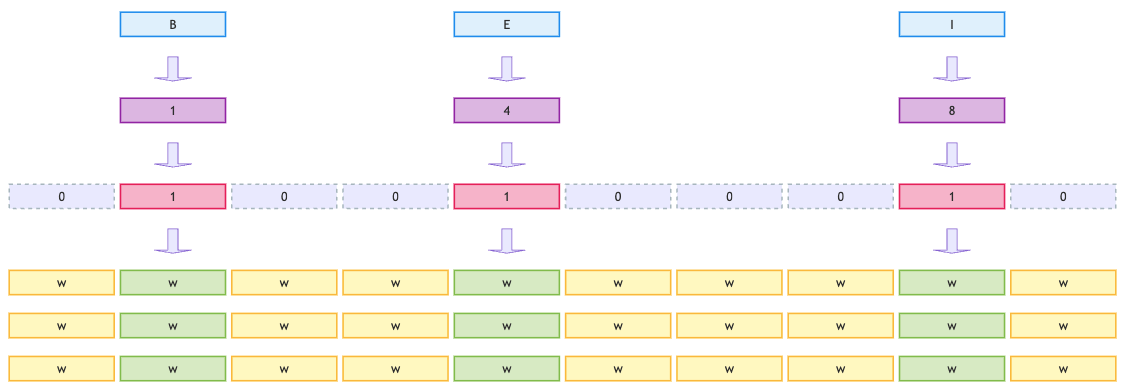
First, we can do this with a linear layer. We set the layer’s input feature dimension in_size to 10,000 and its output feature dimension out_size to 128. The weight matrix then has the shape (128, 10000), where each row is one neuron producing one output value;
Going one step further, each input is a one-hot encoding, with exactly one position equal to 1. The result is therefore simply the column of the weight matrix at that position. If the input is the one-hot vectors of a piece of text, the result is the few columns at the corresponding positions;
So we do not actually need the one-hot encoding at all. We can use the index encoding directly as an index and cut the matching column (or columns) out of the weight matrix, without any vector computation. We call this method embedding.

Bag-of-words embedding: the index encodings select the matching word vectors from the embedding weight matrix, which are then merged into a single vector

Figure: Bag-of-words embedding

from abc import ABC, abstractmethod

import numpy as np

np.random.seed(42)

Tensor¶

class Tensor:

    def __init__(self, data):
        self.data = np.array(data)
        self.grad = np.zeros_like(self.data)
        self.gradient_fn = None
        self.parents = set()

    def backward(self):
        if self.gradient_fn is not None:
            self.gradient_fn()

        for p in self.parents:
            p.backward()

    def __str__(self):
        return f'Tensor({self.data})'

Dataset¶

Abstract class¶

class Dataset(ABC):

    def __init__(self, batch_size=1):
        self.batch_size = batch_size
        self.load()
        self.train()

    @abstractmethod
    def load(self):
        pass

    def train(self):
        self.data = self.train_data

    def eval(self):
        self.data = self.test_data

    def all(self):
        x, y = self.data
        return Tensor(x), Tensor(y)

    def __len__(self):
        x, *_ = self.data
        return len(x) // self.batch_size

    def __getitem__(self, index):
        s = slice(index * self.batch_size, (index + 1) * self.batch_size)
        x, y = self.data
        return Tensor(x[s]), Tensor(y[s])

Character-encoding dataset¶

We no longer need one-hot encoding to build the feature $x$ . Instead, we directly use the set of index encodings of the input text, that is, the token array. The job of encoding is taken over by a separate embedding layer.

The label $y$ still uses one-hot encoding, to match the multi-class classification task.

class CharDataset(Dataset):

    def __init__(self, filename, batch_size=1, context_size=64, stride=None, split=0.9):
        self.filename = filename
        self.context_size = context_size
        self.stride = stride if stride is not None else context_size // 2
        self.split = split
        super().__init__(batch_size)

    def load(self):
        with open(self.filename, encoding="utf-8") as f:
            text = f.read()

        self.vocab = sorted(set(text))
        self.vocab_size = len(self.vocab)
        self.stoi = {ch: i for i, ch in enumerate(self.vocab)}
        self.itos = {i: ch for i, ch in enumerate(self.vocab)}
        self.tokens = self.encode(text)

        split = int(len(self.tokens) * self.split)
        self.train_data = self._pack(self.tokens[:split])
        self.test_data = self._pack(self.tokens[split:])

    def _pack(self, tokens):
        onehot = np.eye(self.vocab_size)
        x, y = [], []
        for i in range(0, len(tokens) - self.context_size - 1, self.stride):
            # Feature: array of index encodings
            x.append(tokens[i: i + self.context_size])
            # Label: one-hot encoding
            y.append(onehot[tokens[i + self.context_size]])
        return x, y

    def encode(self, symbols):
        return [self.stoi[s] for s in symbols]

    def decode(self, tokens):
        return "".join(self.itos[t] for t in tokens)

Model¶

Abstract layer¶

class Layer(ABC):

    def __call__(self, x: Tensor):
        return self.forward(x)

    @abstractmethod
    def forward(self, x: Tensor):
        pass

    @property
    def parameters(self):
        return []

Linear layer¶

class Linear(Layer):

    def __init__(self, in_size, out_size):
        self.weight = Tensor(np.random.randn(out_size, in_size) * np.sqrt(2 / in_size))
        self.bias = Tensor(np.zeros(out_size))

    def forward(self, x: Tensor):
        p = Tensor(x.data @ self.weight.data.T + self.bias.data)

        def gradient_fn():
            self.weight.grad += p.grad.T @ x.data
            self.bias.grad += np.sum(p.grad, axis=0)
            x.grad += p.grad @ self.weight.data

        p.gradient_fn = gradient_fn
        p.parents = [x]
        return p

    @property
    def parameters(self):
        return [self.weight, self.bias]

Sequential layer¶

class Sequential(Layer):

    def __init__(self, layers):
        self.layers = layers

    def forward(self, x: Tensor):
        for l in self.layers:
            x = l(x)
        return x

    @property
    def parameters(self):
        return [p for l in self.layers for p in l.parameters]

Embedding layer¶

In essence, the embedding layer is a linear layer designed specially for encoded vectors. The idea is to replace the huge but sparse one-hot vector with a much smaller dense vector.

Forward propagation (table lookup): the input of the embedding layer is the token array (the array of index encodings) of the input text. Forward propagation uses this array of index encodings to look up the weight matrix and takes out the rows at the corresponding positions. Each row of weights is the dense vector we want, called a word vector;
Backpropagation: as with a linear layer, the weight matrix of the embedding layer must be optimized during training. The difference is that forward propagation uses only a few specific rows of weights, so backpropagation only needs to accumulate gradients onto those rows (if the same token appears several times, its gradient is accumulated several times).

💡 Tip: When we derived this with a linear layer above, the weight matrix had the shape (128, 10000) and we took out columns. The weight matrix of the embedding layer is stored transposed, as (vocabulary size, embedding size), so looking it up by index takes out rows. The two approaches are equivalent.

💡 Tip: Another difference from a linear layer is that the embedding layer has no bias parameter. Its forward propagation is a table lookup, with no weighted sum.

class Embedding(Layer):

    def __init__(self, vocab_size, embedding_size, std=0.02):
        super().__init__()
        self.weight = Tensor(np.random.randn(vocab_size, embedding_size) * std)

    def forward(self, x: Tensor):
        # Look up the table and create the embedding tensor
        p = Tensor(self.weight.data[x.data])

        # Gradient (closure) function of the embedding tensor
        def gradient_fn():
            np.add.at(self.weight.grad, x.data, p.grad)

        p.gradient_fn = gradient_fn
        # Parent list of the embedding tensor
        p.parents = [self.weight]
        return p

    @property
    def parameters(self):
        return [self.weight]

Mean pooling layer¶

After the embedding layer has looked up the table, a piece of text becomes a set of word vectors (one row for each character).

The mean pooling layer averages all the word vectors that were taken out and merges them into a single vector. This vector contains the information of the whole piece of text. The purpose is to connect to a multi-layer network model along the data dimension, and another benefit is that text of different lengths can be handled.

💡 Tip: Like a bag of words, the result of merging by mean pooling loses the word order information of the text.

class MeanPool(Layer):

    def forward(self, x: Tensor):
        # Create the output tensor
        p = Tensor(np.mean(x.data, axis=1))

        # Gradient (closure) function of the output tensor
        def gradient_fn():
            x.grad += p.grad[:, None, :] / x.data.shape[1]

        p.gradient_fn = gradient_fn
        # Parent list of the output tensor
        p.parents = [x]
        return p

Activation functions¶

Rectified linear unit (ReLU)¶

class ReLU(Layer):

    def forward(self, x: Tensor):
        a = Tensor(np.maximum(0, x.data))

        def gradient_fn():
            x.grad += a.grad * (a.data > 0)

        a.gradient_fn = gradient_fn
        a.parents = [x]
        return a

Softmax¶

class Softmax(Layer):

    def __init__(self, axis=-1):
        super().__init__()
        self.axis = axis

    def forward(self, x: Tensor):
        exp = np.exp(x.data - np.max(x.data, axis=self.axis, keepdims=True))
        a = Tensor(exp / np.sum(exp, axis=self.axis, keepdims=True))

        def gradient_fn():
            grad = np.sum(a.data * a.grad, axis=self.axis, keepdims=True)
            x.grad += a.data * (a.grad - grad)

        a.gradient_fn = gradient_fn
        a.parents = [x]
        return a

Loss function (mean squared error)¶

class MSELoss:

    def __call__(self, p: Tensor, y: Tensor):
        return self.loss(p, y)

    def loss(self, p: Tensor, y: Tensor):
        mse = Tensor(np.mean(np.square(y.data - p.data)))

        def gradient_fn():
            p.grad += -2 * (y.data - p.data) / y.data.size

        mse.gradient_fn = gradient_fn
        mse.parents = [p]
        return mse

Optimizer (stochastic gradient descent)¶

class SGDOptimizer:

    def __init__(self, parameters, lr):
        self.parameters = parameters
        self.lr = lr

    def zero_grad(self):
        for p in self.parameters:
            p.grad = np.zeros_like(p.data)

    def step(self):
        for p in self.parameters:
            p.data -= p.grad * self.lr

Trainer¶

class Trainer:

    def __init__(self, model, loss_fn, optimizer):
        self.model = model
        self.loss_fn = loss_fn
        self.optimizer = optimizer

    def train(self, dataset, epochs):
        dataset.train()

        for epoch in range(epochs):
            for i in range(len(dataset)):
                feature, label = dataset[i]

                self.optimizer.zero_grad()
                prediction = self.model(feature)
                loss = self.loss_fn(prediction, label)
                loss.backward()
                self.optimizer.step()

    def test(self, dataset):
        dataset.eval()

        feature, label = dataset.all()
        prediction = self.model(feature)
        loss = self.loss_fn(prediction, label)
        return prediction, loss

    def generate(self, dataset, prompt, steps=256):
        tokens = dataset.encode(prompt)

        for _ in range(steps):
            window = tokens[-dataset.context_size:]
            feature = Tensor([window])
            prediction = self.model(feature)

            probs = prediction.data[0] / np.sum(prediction.data[0])
            token = np.random.choice(len(probs), p=probs)
            tokens.append(token)

        return dataset.decode(tokens)

Hyperparameters¶

Learning rate¶

LEARNING_RATE = 0.01

Batch size¶

BATCH_SIZE = 4

Number of epochs¶

EPOCHS = 10

Context size¶

CONTEXT_SIZE = 32

Embedding size¶

The embedding size is the hyperparameter of the embedding layer. It is how small we want to compress the data vector from the vocabulary size.

In real large models, at the time of GPT-3 the vocabulary size was about 50K, and the embedding size ranged from a few hundred to just over ten thousand (12,288 for the largest model). The latest large models have expanded their vocabularies to 100K to 200K, with embedding sizes of around 10K.

EMBEDDING_SIZE = 16

Modeling¶

The feature provided by the dataset has changed from a one-hot bag-of-words vector into a token array (a set of index encodings).

Our network model also gains an embedding layer and a mean pooling layer, whose purpose is to convert and merge the set of index encodings of the feature into one vector, the mean of the embedding weights.

After that comes the usual two-layer network model:

Embedding: the embedding layer, which converts the set of index encodings into a set of embedding vectors;
MeanPool: the mean pooling layer, which compresses these embedding vectors into one vector;
Linear: the hidden layer;
ReLU: the hidden layer activation function;
Linear: the output layer;
Softmax: the output layer activation function, which outputs the probability distribution of the next character.

The shapes of the data through the model are: the feature (batch size, context size), the embedding layer output (batch size, context size, embedding size), the mean pooling layer output (batch size, embedding size), and the final prediction (batch size, vocabulary size).

DATA_FILE = "../../../../data/tinyshakespeare.txt"

dataset = CharDataset(DATA_FILE, BATCH_SIZE, CONTEXT_SIZE)
model = Sequential([
    # Embedding layer
    Embedding(dataset.vocab_size, EMBEDDING_SIZE),
    # Mean pooling layer
    MeanPool(),
    # Hidden layer
    Linear(EMBEDDING_SIZE, EMBEDDING_SIZE * 2),
    # Hidden layer activation function
    ReLU(),
    # Output layer
    Linear(EMBEDDING_SIZE * 2, dataset.vocab_size),
    # Output layer activation function
    Softmax()
])
loss_fn = MSELoss()
optimizer = SGDOptimizer(model.parameters, lr=LEARNING_RATE)
trainer = Trainer(model, loss_fn, optimizer)

Training¶

trainer.train(dataset, EPOCHS)

Evaluation¶

prediction, loss = trainer.test(dataset)
print(f'prediction:\t{prediction.data.shape}\nloss:\t{loss}')

prediction:	(6970, 65)
loss:	Tensor(0.015120499995513398)

Inference¶

print(trainer.generate(dataset, prompt="ROMEO:"))

ROMEO:tLjtp;xLJ$S,DHnrGqqk3gwfITdU-Hnq.wIeknwHq.gjfDr:$hSqM:pX?hUaRooh,pegKsi-Ns!xfcEDwGlM.
WyLKJVPsUU.yD&eaOOm?odOQDkUHazPuJ$AOB
upj:-&ivP-UJLbh,!zC$?!MnJQeUqr
lRzSzkDWzq,hJ
NCoIo
GCC&?XFOLrtTI,w$GGH:m-c-&t?oW&xCq:q
Ulvtos?FFLMW:g:HUmjd3W'LO!ExwK!;Mw.k,yLlJc?3v

In this chapter, we upgraded the representation of text from one-hot encoding to embedding vectors.

The purpose was to reduce the amount of data. But it does not noticeably improve the quality of inference: like a bag of words, mean pooling still does not use the word order of the text. The inference result shows this, since the output is still meaningless gibberish.

Exercises¶

Try changing the embedding size, for example reducing it to 8 or increasing it to 128, and observe how it affects the speed and results of training and inference.